5.2. Diagonalization - EECS 245 Course Notes

The Eigenvalue Decomposition¶

Recall that if $A$ is an $n \times n$ matrix, then $A$ has $n$ eigenvalues, it’s just that some of the eigenvalues may be complex (leading to complex-valued eigenvectors), and some eigenvalues may be repeated. These $n$ eigenvalues are all solutions to the characteristic polynomial of $A$ ,

p(\lambda) = \text{det}(A - \lambda I)

The corresponding eigenvectors are the solutions to the system of equations $(A - \lambda I) \vec v = \vec 0$ .

Suppose $A$ has $n$ linearly independent eigenvectors $\vec v_1, \vec v_2, \cdots, \vec v_n$ , with eigenvalues $\lambda_1, \lambda_2, \cdots, \lambda_n$ . What I’m about to propose next will seem a little arbitrary, but bear with me – you’ll see the power of this idea shortly. What happens if we multiply $A$ by a matrix, say $V$ , whose columns are the eigenvectors of $A$ ?

\begin{align*} AV &= A \begin{bmatrix} | & | && | \\ \vec v_1 & \vec v_2 & \cdots & \vec v_n \\ | & | && | \end{bmatrix} \\ &= \begin{bmatrix} | & | && | \\ A\vec v_1 & A\vec v_2 & \cdots & A\vec v_n \\ | & | && | \end{bmatrix} \\ &= \begin{bmatrix} | & | && | \\ \lambda_1 \vec v_1 & \lambda_2 \vec v_2 & \cdots & \lambda_n \vec v_n \\ | & | && | \end{bmatrix} \end{align*}

$AV$ is a matrix whose columns are eigenvectors of $A$ , each scaled by the corresponding eigenvalue! Is there another way to write the last line above?

\begin{align*} AV &= \begin{bmatrix} | & | && | \\ \lambda_1 \vec v_1 & \lambda_2 \vec v_2 & \cdots & \lambda_n \vec v_n \\ | & | && | \end{bmatrix} \\ &= \begin{bmatrix} | & | && | \\ \vec v_1 & \vec v_2 & \cdots & \vec v_n \\ | & | && | \end{bmatrix} \begin{bmatrix} \lambda_1 & 0 & \cdots & 0 \\ 0 & \lambda_2 & \cdots & 0 \\ \vdots & \vdots & \ddots & \vdots \\ 0 & 0 & \cdots & \lambda_n \end{bmatrix} \\ &= V \Lambda \end{align*}

Here, $\mathcal{\Lambda}$ (the capitalized Greek letter for $\mathbf{\lambda}$ ) is a diagonal matrix of eigenvalues in the same order as the eigenvectors in $V$ .

AV = V \Lambda

We can take this a step further. If $V$ is invertible – which it is here, since we assumed $A$ has $n$ linearly independent eigenvectors – then we can multiply both sides of the equation above by $V^{-1}$ on the right to get

A = V \Lambda V^{-1}

The existence of this decomposition is contingent on $V$ being invertible, which happens when $A$ has $n$ linearly independent eigenvectors. If $A$ doesn’t have “enough” eigenvectors, then $V$ wouldn’t be invertible, and we wouldn’t be able to decompose $A$ in this way.

Diagonalizable Matrices¶

Definition: Diagonalizable Matrix

A matrix $A$ is diagonalizable if it has an eigenvalue decomposition

A = V \Lambda V^{-1}

using the same definitions of $V$ and $\mathcal{\Lambda}$ above. $A$ is diagonalizable if and only if it has $n$ linearly independent eigenvectors (which allows for $V$ to be invertible). Otherwise, $A$ is not diagonalizable, and is sometimes called defective.

Often, $A$ is defined to be diagonalizable if and only if it can be written in the form

A = PDP^{-1}

where $P$ is some invertible matrix and $D$ is some diagonal matrix. This is a general definition of diagonalizability. But, the only matrices that can be written in $A = PDP^{-1}$ have eigenvalue decompositions and vice versa. The eigenvalue decomposition tells you how to actually diagonalize $A$ .

A First Example¶

Let’s start with a familiar example, $A = \begin{bmatrix} 1 & 2 \\ 2 & 1 \end{bmatrix}$ , which was the first example we saw in Chapter 5.1. $A$ has eigenvalues $\lambda_1 = 3$ and $\lambda_2 = -1$ , and corresponding eigenvectors $\vec v_1 = \begin{bmatrix} 1 \\ 1 \end{bmatrix}$ and $\vec v_2 = \begin{bmatrix} 1 \\ -1 \end{bmatrix}$ . These eigenvectors are linearly independent, so $A$ is diagonalizable, and we can write

V = \begin{bmatrix} 1 & 1 \\ 1 & -1 \end{bmatrix}, \qquad \Lambda = \begin{bmatrix} 3 & 0 \\ 0 & -1 \end{bmatrix}

which tells us that

V \Lambda V^{-1} = \begin{bmatrix} 1 & 1 \\ 1 & -1 \end{bmatrix} \begin{bmatrix} 3 & 0 \\ 0 & -1 \end{bmatrix} \begin{bmatrix} 1/2 & 1/2 \\ 1/2 & -1/2 \end{bmatrix} = \begin{bmatrix} 1 & 2 \\ 2 & 1 \end{bmatrix} = A

Let’s check with numpy.

import numpy as np

V = np.array([[1, 1], 
              [1, -1]])

Lambda = np.diag([3, -1]) # New tool.
V_inv = np.linalg.inv(V)
V @ Lambda @ V_inv # The same as A!

array([[1., 2.],
       [2., 1.]])

Is this decomposition unique? No, because we could have chosen a different set of eigenvectors, or wrote them in a different order (in which case $\mathcal{\Lambda}$ would be different). We’ll keep the eigenvectors in the same order, but instead let’s consider

V = \begin{bmatrix} 2 & -5 \\ 2 & 5 \end{bmatrix}

which is also a valid eigenvector matrix for $A$ . (Remember that any scalar multiple of an eigenvector is still an eigenvector!)

It is still true that $A = V \Lambda V^{-1}$ . This may seem a little unbelievable (I wasn’t convinced at first), but remember that $V^{-1}$ “undoes” any changes in scaling we introduce to $V$ .

V \Lambda V^{-1} = \begin{bmatrix} 2 & -5 \\ 2 & 5 \end{bmatrix} \begin{bmatrix} 3 & 0 \\ 0 & -1 \end{bmatrix} \begin{bmatrix} 1/4 & 1/4 \\ -1/10 & 1/10 \end{bmatrix} = \begin{bmatrix} 1 & 2 \\ 2 & 1 \end{bmatrix} = A

V = np.array([[2, -5], 
              [2, 5]])
              
Lambda = np.diag([3, -1])
V_inv = np.linalg.inv(V)
V @ Lambda @ V_inv # Same as above!

array([[1., 2.],
       [2., 1.]])

Key Applications¶

Rightfully, you might be asking what the point of this is. There are (at least) two main uses of the eigenvalue decomposition.

Application 1: Matrix Powers¶

The first is that it makes it easy to compute powers of $A$ , which we know is a useful concept in understanding the long-run behavior of a Markov chain.

Suppose $A = V \Lambda V^{-1}$ . Then,

A^2 = (V \Lambda V^{-1})(V \Lambda V^{-1}) = V \Lambda (V^{-1}V) \Lambda V^{-1} = V \Lambda^2 V^{-1}

What does this say about $A^3$ ?

A^3 = (V \Lambda V^{-1})(V \Lambda V^{-1})(V \Lambda V^{-1}) = V \Lambda (V^{-1}V) \Lambda (V^{-1}V) \Lambda V^{-1} = V \Lambda^3 V^{-1}

In general, if $k$ is a positive integer,

\boxed{A^k = V \Lambda^k V^{-1}}

So, to compute $A^k$ , we don’t need to multiply $k$ matrices together (which would be a computational nightmare for large $k$ ). Instead, all we need to do is compute $V \Lambda^k V^{-1}$ . And remember, $\mathcal{\Lambda}$ is a diagonal matrix, so computing $\Lambda^k$ is easy: we just raise the diagonal entries to the power in question.

For example, $A^{10} = \begin{bmatrix} 1 & 2 \\ 2 & 1 \end{bmatrix}^{10}$ is

\begin{align*} A^{10} &= V \Lambda^{10} V^{-1} \\ &= \begin{bmatrix} 1 & 1 \\ 1 & -1 \end{bmatrix} \begin{bmatrix} 3^{10} & 0 \\ 0 & (-1)^{10} \end{bmatrix} \begin{bmatrix} 1/2 & 1/2 \\ 1/2 & -1/2 \end{bmatrix} \\ &= \begin{bmatrix} 1 & 1 \\ 1 & -1 \end{bmatrix} \begin{bmatrix} 3^{10}/2 & 3^{10}/2 \\1 /2 & -1/2 \end{bmatrix} \\ &= \begin{bmatrix} (3^{10} + 1)/2 & (3^{10} - 1)/2 \\ (3^{10} - 1)/2 & (3^{10} + 1)/2 \end{bmatrix} \end{align*}

Pretty neat!

np.linalg.matrix_power(A, 10)

array([[29525., 29524.],
       [29524., 29525.]])

Application 2: Understanding Linear Transformations¶

Remember that if $A$ is an $n \times n$ matrix, then $f(\vec x) = A \vec x$ is a linear transformation from $\mathbb{R}^n$ to $\mathbb{R}^n$ . But, if $A = V \Lambda V^{-1}$ , then

f(\vec x) = A \vec x = V \Lambda V^{-1} \vec x

This allows us to understand the effect of $f$ on $\vec x$ in three stages. Remember that $V$ ’s columns are the eigenvectors of $A$ , so the act of multiplying a vector $\vec y$ by $V$ is equivalent to taking a linear combination of $V$ ’s columns ( $A$ ’s eigenvectors) using the weights in $\vec y$ .

V \vec y = \begin{bmatrix} | & | & \cdots & | \\ \vec v_1 & \vec v_2 & \cdots & \vec v_n \\ | & | & \cdots & | \end{bmatrix} \begin{bmatrix} y_1 \\ y_2 \\ \vdots \\ y_n \end{bmatrix} = y_1 \vec v_1 + y_2 \vec v_2 + \cdots + y_n \vec v_n

For example, $V \begin{bmatrix} 3 \\ -4 \end{bmatrix}$ says take 3 of the first eigenvector, and -4 of the second eigenvector, and add them together to get a new vector. If $V \begin{bmatrix} 3 \\ -4 \end{bmatrix} = \begin{bmatrix} 1 \\ 2 \end{bmatrix}$ , this says that taking 3 of the first eigenvector and -4 of the second eigenvector is the same as taking 1 of the first standard basis vector, $\begin{bmatrix} 1 \\ 0 \end{bmatrix}$ and 2 of the second standard basis vector, $\begin{bmatrix} 0 \\ 1 \end{bmatrix}$ .

Intuitively, think of $V$ as a matrix that takes in “amounts of each eigenvector” and outputs “amounts of each standard basis vector”, where the standard basis vectors are the columns of $I$ .

So, if

V: \text{eigenvector amounts} \to \text{standard basis vector amounts}

then $V^{-1}$ does the opposite, and maps

V^{-1}: \text{standard basis vector weights} \to \text{eigenvector amounts}

i.e. multiplying $V^{-1}$ by $\vec x$ expresses $\vec x$ as a linear combination of the eigenvectors of $A$ . If $\vec z$ is the output of $V^{-1} \vec x$ , then $\vec x = V \vec z$ , meaning $\vec z$ contains the amounts of each eigenvector needed to produce $\vec x$ .

(This is non-standard notation, since $V$ is not a function and $\text{eigenvector amounts}$ and $\text{standard basis vector amounts}$ are not sets but concepts, but I hope this helps convey the role of $V$ and $V^{-1}$ in this context.)

Taking a step back, recall

f(\vec x) = A \vec x = V \Lambda V^{-1} \vec x

What this is saying is $f$ does three things:

First, it takes $\vec x$ and expresses it as a linear combination of the eigenvectors of $A$ , which is $V^{-1} \vec x$ . (This contains the “amounts of each eigenvector” needed to produce $\vec x$ .)
Then, it takes that linear combination $V^{-1} \vec x$ and scales each eigenvector by its corresponding eigenvalue, i.e. it scales or stretches each eigenvector by a different amount. Remember that diagonal matrices only scale, they don’t do anything else!
Finally, it takes the resulting scaled vector $\Lambda V^{-1} \vec x$ and expresses it as a linear combination of the standard basis vectors, i.e. it combines the correct amounts of the stretched eigenvectors to get the final result.

\underbrace{\text{express in eigenvector basis}}_{\text{multiply by } V^{-1}} \to \underbrace{\text{scale eigenvectors}}_{\text{multiply by } \Lambda} \to \underbrace{\text{express in standard basis}}_{\text{multiply by } V}

This is better understood visually, as you’ll see in the Symmetric Matrices and the Spectral Theorem section below.

Examples¶

Example: Non-Diagonalizable Matrices¶

Most matrices we’ve seen in Chapter 5.1 and here so far in Chapter 5.2 have been diagonalizable. I’ve tried to shield you from the messy world of non-diagonalizable matrices until now, but we’re ready to dive deeper.

Consider $A = \begin{bmatrix} 1 & 1 \\ 0 & 1 \end{bmatrix}$ . The characteristic polynomial of $A$ is

p(\lambda) = \text{det}(A - \lambda I) = \text{det} \begin{bmatrix} 1 - \lambda & 1 \\ 0 & 1 - \lambda \end{bmatrix} = (1 - \lambda)^2

which has a double root of $\lambda = 1$ . So, $A$ has a single eigenvalue $\lambda = 1$ . What are all of $A$ ’s eigenvectors? They’re solutions to $A \vec v = 1 \vec v$ , i.e. $(A - I) \vec v = \vec 0$ . Let’s look at the null space of $A - I$ :

A - I = \begin{bmatrix} 1 - 1 & 1 \\ 0 & 1 - 1 \end{bmatrix} = \begin{bmatrix} 0 & 1 \\ 0 & 0 \end{bmatrix}

The null space of $A - I$ is spanned by the single vector $\begin{bmatrix} 1 \\ 0 \end{bmatrix}$ . So, $A$ has a single line of eigenvectors, spanned by $\vec v_1 = \begin{bmatrix} 1 \\ 0 \end{bmatrix}$ .

So, does $A$ have an eigenvalue decomposition? No, because we don’t have enough eigenvectors to form $V$ . If we try and form $V$ by using $\vec v_1$ in the first column and a column of zeros in the second column, we’d have

V = \begin{bmatrix} 1 & 0 \\ 0 & 0 \end{bmatrix}

but this is not an invertible matrix, so $V$ is not invertible, and we can’t write $A = V \Lambda V^{-1}$ . $A$ is not diagonalizable! This means that it’s harder to interpret $A$ as a linear transformation through the lens of eigenvectors, and it’s harder to understand the long-run behavior of $A^k \vec x$ for an arbitrary $\vec x$ .

Let me emphasize what I mean by $A$ needing to have $n$ linearly independent eigenvectors. Above, we found that $\begin{bmatrix} 1 \\ 0 \end{bmatrix}$ is an eigenvector of $A$ , which means that any scalar multiple of $\begin{bmatrix} 1 \\ 0 \end{bmatrix}$ is also an eigenvector of $A$ . But, the matrix

\begin{bmatrix} 1 & 2 \\ 0 & 0 \end{bmatrix}

is not invertible, meaning it can’t be the $V$ in $A = V \Lambda V^{-1}$ .

Example: The Identity Matrix¶

The $2 \times 2$ identity matrix $I = \begin{bmatrix} 1 & 0 \\ 0 & 1 \end{bmatrix}$ has the characteristic polynomial $p(\lambda) = (\lambda - 1)^2$ . So, $I$ has a single eigenvalue $\lambda = 1$ , just like the last example.

But, $\lambda = 1$ corresponds to two different eigenvector directions! I can pick any two linearly independent vectors in $\mathbb{R}^2$ and they’ll both be eigenvectors for $I$ . For example, let $\vec v_1 = \begin{bmatrix} 1 \\ -3 \end{bmatrix}$ and $\vec v_2 = \begin{bmatrix} 11 \\ 98 \end{bmatrix}$ , meaning

V = \begin{bmatrix} 1 & 11 \\ -3 & 98 \end{bmatrix}

The matrix $\mathcal{\Lambda}$ is just $\begin{bmatrix} 1 & 0 \\ 0 & 1 \end{bmatrix}$ which is the same as $I$ itself. This means that as long as $V$ is invertible (i.e. as long as I pick two linearly independent vectors in $\mathbb{R}^2$ ),

V \Lambda V^{-1} = V I V^{-1} = V V^{-1} = I

which means that indeed, $I$ is diagonalizable. (Any matrix that is diagonal to begin with is diagonalizable: in $A = PDP^{-1}$ , $P$ is just the identity matrix.)

If you’d rather look at this example through the lens of solving systems of equations, an eigenvector $\vec v = \begin{bmatrix} a \\ b \end{bmatrix}$ of $I$ with eigenvalue $\lambda = 1$ satisfies

I \vec v = \begin{bmatrix} 1 & 0 \\ 0 & 1 \end{bmatrix} \begin{bmatrix} a \\ b \end{bmatrix} = \begin{bmatrix} a \\ b \end{bmatrix} = 1 \begin{bmatrix} a \\ b \end{bmatrix}

But, as a system this just says $a = a$ and $b = b$ , which is true for any $\vec v$ . Think of $a$ and $b$ both as independent variables; the set of possible $\vec v$ ’s, then, is two dimensional (and is all of $\mathbb{R}^2$ ).

Example: Non-Invertible Matrices¶

Let $A = \begin{bmatrix} 1 & 2 \\ 2 & 4 \end{bmatrix}$ .

$A$ is not invertible (column 2 is double column 1), so it has an eigenvalue of $\lambda_1 = 0$ , which corresponds to the eigenvector $\vec v_1 = \begin{bmatrix} -2 \\ 1 \end{bmatrix}$ .
It also has an eigenvalue of $\lambda_2 = 5$ , corresponding to the eigenvector $\vec v_2 = \begin{bmatrix} 1 \\ 2 \end{bmatrix}$ . (Remember, the quick way to spot this eigenvalue is to remember that the sum of the eigenvalues of $A$ is equal to the trace of $A$ , which is $1 + 4 = 5$ ; since 0 is an eigenvalue, the other eigenvalue must be 5.)

Does $A$ have an eigenvalue decomposition? Let’s see if anything goes wrong when we try and construct the eigenvector matrix $V$ and the diagonal matrix $\mathcal{\Lambda}$ and multiplying $V \Lambda V^{-1}$ .

V = \begin{bmatrix} -2 & 1 \\ 1 & 2 \end{bmatrix}, \qquad \Lambda = \begin{bmatrix} 0 & 0 \\ 0 & 5 \end{bmatrix}

V \Lambda V^{-1} = \begin{bmatrix} -2 & 1 \\ 1 & 2 \end{bmatrix} \begin{bmatrix} 0 & 0 \\ 0 & 5 \end{bmatrix} \begin{bmatrix} -2/5 & 1/5 \\ 1/5 & 2/5 \end{bmatrix} = \begin{bmatrix} 1 & 2 \\ 2 & 4 \end{bmatrix}

Everything worked out just fine! $A$ is diagonalizable, even though it’s not invertible.

Algebraic and Geometric Multiplicity¶

As we saw in an earlier example, the matrix $\begin{bmatrix} 1 & 1 \\ 0 & 1 \end{bmatrix}$ does not have two linearly independent eigenvectors, and so is not diagonalizable. I’d like to dive deeper into identifying when a matrix is diagonalizable.

Activity 1

Suppose an $n \times n$ matrix $A$ has the characteristic polynomial

p(\lambda) = (\lambda + 1)^2 \lambda (\lambda - 1)^3 (\lambda - 4)^2 (\lambda - 5) (\lambda - 12)^2

What is $n$ (i.e. the number of rows/columns of $A$ )?
What is the determinant of $A$ ?
What are all of $A$ ’s eigenvalues and their algebraic multiplicities?

Solution

$n$ is equal to the sum of the exponents of the polynomial, which is $2 + 1 + 3 + 2 + 1 + 2 = 11$ . Remember that $p(\lambda)$ is a polynomial of degree $n$ .
The determinant of $A$ is the product of the eigenvalues. Notice that $p(\lambda)$ has a factor of $\lambda$ , i.e. $p(0) = 0$ , meaning 0 is an eigenvalue, so $\text{det}(A) = 0$ .
$A$ has eigenvalues:
- -1 with multiplicity $\text{AM}(-1) = 2$
- 0 with multiplicity $\text{AM}(0) = 1$
- 1 with multiplicity $\text{AM}(1) = 3$
- 4 with multiplicity $\text{AM}(4) = 2$
- 5 with multiplicity $\text{AM}(5) = 1$
- 12 with multiplicity $\text{AM}(12) = 2$
These algebraic multiplicities come from the exponents of the factors in $p(\lambda)$ .

The algebraic multiplicity of an eigenvalue, as the name suggests, is purely a property of the characteristic polynomial. Alone, they don’t tell us whether or not a matrix is diagonalizable. Instead, we’ll need to look at another form of multiplicity alongside the algebraic multiplicity.

Definition: Eigenspace and Geometric Multiplicity

The eigenspace of an eigenvalue $\mathbf{\lambda}_i$ is the set of all eigenvectors with an eigenvalue of $\mathbf{\lambda}_i$ . Equivalently:

It is the set of all vectors $\vec v$ such that $A \vec v = \lambda_i \vec v$ .
It is the subspace $\text{nullsp}(A - \lambda_i I)$ , though $\vec 0$ (which is in the null space) is not technically an eigenvector.

The geometric multiplicity of $\mathbf{\lambda}$ is the dimension of the eigenspace of $\mathbf{\lambda}$ .

\text{GM}(\lambda_i) = \text{dim}(\text{nullsp}(A - \lambda_i I))

Equivalently, the geometric multiplicity of $\lambda_i$ is the number of linearly independent eigenvectors corresponding to $\mathbf{\lambda}_i$ .

The geometric multiplicity of an eigenvalue can’t be determined from the characteristic polynomial alone – instead, it involves finding $\text{nullsp}(A - \lambda_i I)$ and finding its dimension, i.e. the number of linearly independent vectors needed to span it. But in general,

1 \leq \text{GM}(\lambda_i) \leq \text{AM}(\lambda_i)

Think of the algebraic multiplicity of an eigenvalue as the “potential” number of linearly independent eigenvectors for an eigenvalue, sort of like the number of slots we have for that eigenvalue. The geometric multiplicity, on the other hand, is the number of linearly independent eigenvectors we actually have for that eigenvalue. As we’ll see in the following examples, when the geometric multiplicity is less than the algebraic multiplicity for any eigenvalue, the matrix in question is not diagonalizable.

In each of the following matrices $A$ , we’ll

Find the algebraic multiplicity of each of $A$ ’s eigenvalues.
For each eigenvalue, find the geometric multiplicity and a basis for the eigenspace.
Conclude whether $A$ is diagonalizable.

As usual, attempt these examples on your own first before peeking at the solutions.

A First Example¶

A = \begin{bmatrix} 1 & 1 & 0 \\ 0 & 1 & 1 \\ 0 & 0 & 1 \end{bmatrix}

We’ll walk through this one together.

First, we’ll find the characteristic polynomial of $A$ :
$p(\lambda) = \text{det}(A - \lambda I) = \begin{vmatrix} 1 - \lambda & 1 & 0 \\ 0 & 1 - \lambda & 1 \\ 0 & 0 & 1 - \lambda \end{vmatrix} = (1 - \lambda)^3$
(You should practice quickly finding the characteristic polynomial of a $3 \times 3$ matrix; Chapter 5.1 has relevant examples.)
This tells us that $A$ has a single eigenvalue $\lambda = 1$ , with algebraic multiplicity $\boxed{\text{AM}(1) = 3}$ .
The geometric multiplicity of $\lambda = 1$ is $\text{dim}(\text{nullsp}(A - I))$ . Let’s look at $A - I$ :
$A - I = \begin{bmatrix} 0 & 1 & 0 \\ 0 & 0 & 1 \\ 0 & 0 & 0 \end{bmatrix}$
$A-I$ has rank 2, so $\text{dim}(\text{nullsp}(A - I)) = 3 - 2 = 1$ (from the rank-nullity theorem), so the geometric multiplicity of $\lambda = 1$ is $\boxed{\text{GM}(1) = 1}$ .
The vector $\vec v_1 = \begin{bmatrix} 1 \\ 0 \\ 0 \end{bmatrix}$ is an eigenvector for $\lambda = 1$ , and so is any scalar multiple of $\vec v_1$ ; I found this by noticing that the first column of $A-I$ is all zeros. So,
$\boxed{\text{nullsp}(A - I) = \text{span} \left( \left\{ \begin{bmatrix} 1 \\ 0 \\ 0 \end{bmatrix} \right\} \right)}$
Since $\text{GM}(1) = 1 < \text{AM}(1) = 3$ , $A$ is not diagonalizable. $A$ only has one linearly independent eigenvector!

Now, it’s your turn.

Example: Adjacency Matrices¶

A = \begin{bmatrix} 0.8 & 0.3 \\ 0.2 & 0.7 \end{bmatrix}

(This is the same adjacency matrix we introduced in Chapter 5.1, Part 2.)

Solution

In Chapter 5.1, Part 2, we found that $A$ has eigenvalues $\lambda_1 = 1$ and $\lambda_2 = 0.5$ , but we’ll find the characteristic polynomial again for clarity:
$\begin{align*} p(\lambda) &= \det(A - \lambda I) \\ &= \begin{vmatrix} 0.8 - \lambda & 0.3 \\ 0.2 & 0.7 - \lambda \end{vmatrix} \\ &= (0.8 - \lambda)(0.7 - \lambda) - (0.3)(0.2) \\ &= \lambda^2 - 1.5\lambda + 0.5 \\ &= (1 - \lambda)(0.5 - \lambda) \end{align*}$
So, the eigenvalues are $\lambda_1 = 1$ and $\lambda_2 = 0.5$ , each with algebraic multiplicity $\boxed{\text{AM}(1) = \text{AM}(0.5) = 1}$ .
The fact that $A$ has two distinct eigenvalues alone tells us that $A$ is diagonalizable, since each eigenvalue has exactly one independent eigenvector (which really means a line of eigenvectors, or a 1-dimensional eigenspace) and eigenvectors for different eigenvalues are always linearly independent. Let’s find those eigenvectors to be sure.
- For $\lambda_1 = 1$ , we solve $(A - I) \vec v = \vec 0$ :
  $A - I = \begin{bmatrix} -0.2 & 0.3 \\ 0.2 & -0.3 \end{bmatrix}$
  The null space of this matrix is spanned by $\begin{bmatrix} 3 \\ 2 \end{bmatrix}$ , so $\boxed{\text{nullsp}(A - I) = \text{span} \left( \left\{ \begin{bmatrix} 3 \\ 2 \end{bmatrix} \right\} \right)}$ and $\boxed{\text{GM}(1) = 1}$ .
- For $\lambda_2 = 0.5$ , we solve $(A - 0.5I) \vec v = \vec 0$ :
  $A - 0.5I = \begin{bmatrix} 0.3 & 0.3 \\ 0.2 & 0.2 \end{bmatrix}$
  The null space of this matrix is spanned by $\begin{bmatrix} -1 \\ 1 \end{bmatrix}$ , so $\boxed{\text{nullsp}(A - 0.5I) = \text{span} \left( \left\{ \begin{bmatrix} -1 \\ 1 \end{bmatrix} \right\} \right)}$ and $\boxed{\text{GM}(0.5) = 1}$ .
Since $A$ has two linearly independent eigenvectors, it is diagonalizable:
$A = V \Lambda V^{-1} = \begin{bmatrix} 3 & -1 \\ 2 & 1 \end{bmatrix} \begin{bmatrix} 1 & 0 \\ 0 & 0.5 \end{bmatrix} \left( \begin{bmatrix} 3 & -1 \\ 2 & 1 \end{bmatrix} \right)^{-1}$

Example: Another Diagonalizable Matrix¶

A = \begin{bmatrix} 2 & 1 & 0 \\ 1 & 2 & 0 \\ 0 & 0 & 3 \end{bmatrix}

This is perhaps the single most comprehensive example!

Solution

The characteristic polynomial of $A$ is
$\begin{align*} p(\lambda) &= \det(A - \lambda I) \\ &= \begin{vmatrix} 2 - \lambda & 1 & 0 \\ 1 & 2 - \lambda & 0 \\ 0 & 0 & 3 - \lambda \end{vmatrix} \\ &= (2 - \lambda)\left((2 - \lambda)(3 - \lambda) - 0 \cdot 0 \right) - 1 \left( (1)(3 - \lambda) - 0 \cdot 0 \right) + 0 \\ &= (2 - \lambda)(2 - \lambda)(3 - \lambda) - (3 - \lambda) \\ &= (3 - \lambda)\left( (2 - \lambda)^2 - 1 \right) \\ &= (3 - \lambda)(\lambda^2 - 4\lambda + 3) \\ &= (3 - \lambda)^2(1 - \lambda) \end{align*}$
So, $A$ has eigenvalues $\lambda_1 = 3$ with $\boxed{\text{AM}(3) = 2}$ and $\lambda_2 = 1$ with $\boxed{\text{AM}(1) = 1}$ .
- For $\lambda_1 = 3$ , we solve $(A - 3I) \vec v = \vec 0$ :
  $A - 3I = \begin{bmatrix} -1 & 1 & 0 \\ 1 & -1 & 0 \\ 0 & 0 & 0 \end{bmatrix}$
  $\text{rank}(A - 3I) = 1$ (since all columns are multiples of $\begin{bmatrix} -1 \\ 1 \\ 0 \end{bmatrix}$ ), so $\text{dim}(\text{nullsp}(A - 3I)) = 3 - 1 = 2$ , which means $\boxed{\text{GM}(3) = 2}$ . At this point, we can conclude that $A$ is diagonalizable! But, let’s find a basis for the eigenspace $\text{nullsp}(A - 3I)$ to be thorough.
  Two linearly independent vectors in $\text{nullsp}(A - 3I)$ are $\begin{bmatrix} 1 \\ 1 \\ 0 \end{bmatrix}$ and $\begin{bmatrix} 0 \\ 0 \\ 1 \end{bmatrix}$ , so $\boxed{\text{nullsp}(A - 3I) = \text{span} \left( \left\{ \begin{bmatrix} 1 \\ 1 \\ 0 \end{bmatrix}, \begin{bmatrix} 0 \\ 0 \\ 1 \end{bmatrix} \right\} \right)}$ . This is just one possible basis for the eigenspace; it’s not the only one.
  What this says is any linear combination of $\begin{bmatrix} 1 \\ 1 \\ 0 \end{bmatrix}$ and $\begin{bmatrix} 0 \\ 0 \\ 1 \end{bmatrix}$ is also an eigenvector for $\lambda = 3$ . For example, $\begin{bmatrix} 2 & 1 & 0 \\ 1 & 2 & 0 \\ 0 & 0 & 3 \end{bmatrix} \begin{bmatrix} -1 \\ -1 \\ 13 \end{bmatrix} = 3 \begin{bmatrix} -1 \\ -1 \\ 13 \end{bmatrix}$ .
- For $\lambda_2 = 1$ , we solve $(A - I) \vec v = \vec 0$ :
  $A - I = \begin{bmatrix} 1 & 1 & 0 \\ 1 & 1 & 0 \\ 0 & 0 & 2 \end{bmatrix}$
  Since $\text{AM}(1) = 1$ , we know that there could only be one linearly independent eigenvector for $\lambda_2 = 1$ , so $\boxed{\text{GM}(1) = 1}$ too. One such eigenvector is $\begin{bmatrix} 1 \\ -1 \\ 0 \end{bmatrix}$ , so $\boxed{\text{nullsp}(A - I) = \text{span} \left( \left\{ \begin{bmatrix} 1 \\ -1 \\ 0 \end{bmatrix} \right\} \right)}$ .
Since $A$ has three linearly independent eigenvectors, it is diagonalizable:
$A = V \Lambda V^{-1} = \begin{bmatrix} 1 & 0 & 1 \\ 1 & 0 & -1 \\ 0 & 1 & 0 \end{bmatrix} \begin{bmatrix} 3 & 0 & 0 \\ 0 & 2 & 0 \\ 0 & 0 & 2 \end{bmatrix} \left( \begin{bmatrix} 1 & 0 & 1 \\ 1 & 0 & -1 \\ 0 & 1 & 0 \end{bmatrix} \right)^{-1}$

Example: Another Non-Diagonalizable Matrix¶

A = \begin{bmatrix} 2 & 1 & 0 \\ 0 & 2 & 0 \\ 0 & 0 & 3 \end{bmatrix}

(Note that this $A$ is almost identical to the $A$ in the previous example, but with a 1 switched to a 0 in the second row.)

Solution

$A$ is upper triangular, so its eigenvalues are the entries on the diagonal: $\lambda_1 = 2$ , $\lambda_2 = 2$ , $\lambda_3 = 3$ . So, $\boxed{\text{AM}(2) = 2}$ and $\boxed{\text{AM}(3) = 1}$ .
- For $\lambda_1 = 2$ , we solve $(A - 2I) \vec v = \vec 0$ :
$A - 2I = \begin{bmatrix} 0 & 1 & 0 \\ 0 & 0 & 0 \\ 0 & 0 & 1 \end{bmatrix}$
$\text{rank}(A-2I) = 2$ , so $\text{dim}(\text{nullsp}(A-2I)) = 1$ , so $\boxed{\text{GM}(2) = 1}$ . At this point, we can conclude that $A$ is not diagonalizable, since $\text{GM}(2) < \text{AM}(2)$ . Noticing that the first column of $A - 2I$ is all zeros, $\vec v_1 = \begin{bmatrix} 1 \\ 0 \\ 0 \end{bmatrix}$ is an eigenvector, and
$\boxed{\text{nullsp}(A-2I) = \text{span} \left( \left\{ \begin{bmatrix} 1 \\ 0 \\ 0 \end{bmatrix} \right\} \right)}$
- For $\lambda_3 = 3$ , we solve $(A - 3I) \vec v = \vec 0$ :
$A - 3I = \begin{bmatrix} -1 & 1 & 0 \\ 0 & -1 & 0 \\ 0 & 0 & 0 \end{bmatrix}$
Using similar logic, $\boxed{\text{GM}(3) = 1}$ and
$\boxed{\text{nullsp}(A-3I) = \text{span} \left( \left\{ \begin{bmatrix} 0 \\ 0 \\ 1 \end{bmatrix} \right\} \right)}$
$A$ only has two linearly independent eigenvectors, one for $\lambda = 2$ and one for $\lambda = 3$ , but is a $3 \times 3$ matrix, and hence its not diagonalizable. (Also, for $\lambda_1 = 2$ , the geometric multiplicity, 1, is less than the algebraic multiplicity, 2, but we need equality for all eigenvalues in order for $A$ to be diagonalizable.)

Activity 3

For each statement, determine whether it is true or false and provide a brief justification. (For false statements, provide a counterexample.)

True or False: If all of $A$ ’s eigenvalues are distinct, then $A$ is diagonalizable.
True or False: If all of $A$ ’s eigenvalues are positive, then $A$ is diagonalizable.
True or False: If $A$ is diagonalizable, then $A$ is invertible.
True or False: If $A$ is invertible, then $A$ is diagonalizable.

Solution

If all of $A$ ’s eigenvalues are distinct, then $A$ is diagonalizable. True. Remember that the minimum possible geometric multiplicity is 1, so if all eigenvalues are distinct, they each have an algebraic and geometric multiplicity of 1. Eigenvectors for different eigenvalues are always linearly independent; think of it this way, an eigenvector can only ever be paired with a single eigenvalue, so eigenvectors for different eigenvalues can’t be linearly dependent. Pairing these two facts, $A$ must have $n$ linearly independent eigenvectors, and so is diagonalizable.
If all of $A$ ’s eigenvalues are positive, then $A$ is diagonalizable. False. The most recent $A$ above had eigenvalues of 2, 2, and 3, all of which are positive, but $A$ was not diagonalizable.
If $A$ is diagonalizable, then $A$ is invertible. False. We saw an example of a diagonalizable matrix that was not invertible above:
$\begin{bmatrix} 1 & 2 \\ 2 & 4 \end{bmatrix} = \underbrace{\begin{bmatrix} 2 & 1 \\ -1 & 2 \end{bmatrix}}_V \underbrace{\begin{bmatrix} 0 & 0 \\ 0 & 5 \end{bmatrix}}_{\Lambda} \underbrace{\left( \begin{bmatrix} 2 & 1 \\ -1 & 2 \end{bmatrix} \right)^{-1}}_{V^{-1}}$
If $A$ is invertible, then $A$ is diagonalizable. False. The most recent $A$ above had eigenvalues of 2, 2, and 3, none of which are 0, meaning $A$ is invertible, but $A$ was not diagonalizable.

Symmetric Matrices and the Spectral Theorem¶

Symmetric matrices – that is, square matrices where $A = A^T$ – behave really nicely through the lens of eigenvectors, and understanding exactly how they work is key to Chapter 5.3, when we generalize beyond square matrices.

If you search for the spectral theorem online, you’ll often just see Statement 4 above; I’ve broken the theorem into smaller substatements to see how they are chained together.

The proof of Statement 1 is beyond our scope, since it involves fluency with complex numbers. If the term “complex conjugate” means something to you, read the proof here – it’s relatively short.
Statement 2 was proved in Lab 11, Activity 5.
I’m not going to cover the proof of Statement 3 here, as I don’t think it’ll add to your learning.

Orthogonal matrices $Q$ satisfy $Q^TQ = QQ^T = I$ , meaning their columns (and rows) are orthonormal, not just orthogonal to one another. The fact that $Q^TQ = QQ^T = I$ means that $Q^T = Q^{-1}$ , so taking the transpose of a matrix is the same as taking its inverse.

So, instead of

A = V \Lambda V^{-1}

we’ve “upgraded” to

A = Q \Lambda Q^T

This is the main takeaway of the spectral theorem: that symmetric matrices can be diagonalized by an orthogonal matrix. Sometimes, $A = Q \Lambda Q^T$ is called the spectral decomposition of $A$ , but all it is is a special case of the eigenvalue decomposition for symmetric matrices.

Visualizing the Spectral Theorem¶

Why do we prefer $Q \Lambda Q^T$ over $V \Lambda V^{-1}$ ? Taking the transpose of a matrix is much easier than inverting it, so actually working with $Q \Lambda Q^T$ is easier.

\underbrace{A = Q \Lambda Q^T \implies A^k = Q \Lambda^k Q^T}_{\text{no inversion needed!}}

But it’s also an improvement in terms of interpretation: remember that orthogonal matrices are matrices that represent rotations. So, if $A$ is symmetric, then the linear transformation $f(\vec x) = A \vec x$ is a sequence of rotations and stretches.

f(\vec x) = A \vec x = Q \Lambda Q^T \vec x

Let’s make sense of this visually. Consider the symmetric matrix $A = \begin{bmatrix} 1 & 2 \\ 2 & 1 \end{bmatrix}$ .

import numpy as np
import plotly.graph_objects as go
from plotly.subplots import make_subplots
from utils import plot_vectors

def plot_unit_square_and_transform(
    A=None, 
    B=None, 
    name_A="A", 
    name_B="B", 
    vdeltax_A=-0.3, 
    vdeltay_A=0.2, 
    vdeltax_B=0.5, 
    vdeltay_B=0, 
    return_fig=False, 
    show_labels=True,
    axis_range=[-3.5, 3.5],
    title=''
):
    """
    Visualize transformation of the unit square and basis vectors under two matrices.
    Left: vectors A u_x and A u_y and parallelogram from A (default is identity -- the unit square and basis)
    Right: vectors B u_x and B u_y and parallelogram from B (default is the input B)
    """
    # Default: left is unit, right is input (legacy)
    if A is None:
        A = np.eye(2)
    if B is None:
        B = np.eye(2)
        
    # Vertices of the unit square
    square = np.array([
        [0, 0],  # A
        [1, 0],  # B
        [1, 1],  # C
        [0, 1],  # D
        [0, 0]   # A (to close the square)
    ])
    square_A = (A @ square.T).T
    square_B = (B @ square.T).T

    # Create subplot figure
    left_title = r"$$" + name_A + r"\vec u_x \text{  and } " + name_A + r"\vec u_y$$" if (name_A and show_labels) else ""
    right_title = r"$$" + name_B + r"\vec u_x \text{  and } " + name_B + r"\vec u_y$$" if (name_B and show_labels) else ""
    fig = make_subplots(
        rows=1, cols=2,
        subplot_titles=(left_title, right_title),
        horizontal_spacing=0.08,
    )

    # Common axis settings
    axis_style = dict(
        showgrid=True,
        gridcolor="#f0f0f0",
        zeroline=False,  # We'll add our own zero lines
        showline=True,
        linecolor="#f0f0f0",
        mirror=True,
        ticks="outside",
        showticklabels=True,
        tickfont=dict(family="Palatino, serif", size=14),
    )
    # Set axis ranges to [-4, 4] for both subplots
    for i in [1, 2]:
        fig.update_xaxes(
            range=axis_range,
            constrain="domain",
            dtick=1,
            **axis_style,
            row=1, col=i
        )
        fig.update_yaxes(
            range=axis_range,
            scaleanchor=f"x{i}",
            dtick=1,
            **axis_style,
            row=1, col=i
        )
    # --- Draw faint 0 grid lines underneath everything else ---
    for i in [1, 2]:
        # Horizontal y=0
        fig.add_shape(
            type="line",
            x0=-4, x1=4, y0=0, y1=0,
            line=dict(color="rgba(170,170,170,0.25)", width=2, dash="solid"),
            row=1, col=i,
            layer="below"
        )
        # Vertical x=0
        fig.add_shape(
            type="line",
            x0=0, x1=0, y0=-4, y1=4,
            line=dict(color="rgba(170,170,170,0.25)", width=2, dash="solid"),
            row=1, col=i,
            layer="below"
        )

    # -- Plot left parallelogram (A unit square) in blue
    fig.add_trace(
        go.Scatter(
            x=square_A[:,0], y=square_A[:,1],
            fill="toself",
            fillcolor="rgba(61,129,246,0.4)",
            line=dict(color="rgba(0,0,0,0)", width=0),  # No perimeter
            name=f"{name_A} square",
            showlegend=False
        ),
        row=1, col=1
    )
    # -- Plot right parallelogram (B unit square) in orange
    fig.add_trace(
        go.Scatter(
            x=square_B[:,0], y=square_B[:,1],
            fill="toself",
            fillcolor="rgba(255,140,0,0.4)",
            line=dict(color="rgba(0,0,0,0)", width=0),
            name=f"{name_B} square",
            showlegend=False
        ),
        row=1, col=2
    )

    # --- Draw vectors using plot_vectors ---
    # Standard basis vectors
    u_x = np.array([1, 0])
    u_y = np.array([0, 1])

    # Left: A u_x, A u_y in #3d81f6
    Au_x = A @ u_x
    Au_y = A @ u_y
    if show_labels:
        left_vecs = [
            (tuple(Au_x), '#3d81f6', rf'${name_A}\vec u_x$'),
            (tuple(Au_y), '#3d81f6', rf'${name_A}\vec u_y$'),
        ]
    else:
        left_vecs = [
            (tuple(Au_x), '#3d81f6', None),
            (tuple(Au_y), '#3d81f6', None),
        ]
    left_fig = plot_vectors(left_vecs, vdeltax=vdeltax_A, vdeltay=vdeltay_A)
    left_fig.update_layout(
        plot_bgcolor="rgba(0,0,0,0)",
        paper_bgcolor="rgba(0,0,0,0)",
        xaxis=dict(visible=False),
        yaxis=dict(visible=False),
        margin=dict(l=0, r=0, t=0, b=0)
    )
    # Add the vector traces to the left subplot
    for trace in left_fig.data:
        fig.add_trace(trace, row=1, col=1)
    # Add the vector annotations to the left subplot, if enabled
    if show_labels:
        for ann in left_fig.layout.annotations:
            if hasattr(ann, "to_plotly_json"):
                ann_dict = ann.to_plotly_json()
            else:
                ann_dict = dict(ann)
            ann_dict = {k: v for k, v in ann_dict.items() if k not in {"xref", "yref", "axref", "ayref"}}
            fig.add_annotation(**ann_dict, row=1, col=1)

    # Right: B u_x, B u_y in orange
    Bu_x = B @ u_x
    Bu_y = B @ u_y
    if show_labels:
        right_vecs = [
            (tuple(Bu_x), 'orange', rf'${name_B}\vec u_x$'),
            (tuple(Bu_y), 'orange', rf'${name_B}\vec u_y$'),
        ]
    else:
        right_vecs = [
            (tuple(Bu_x), 'orange', None),
            (tuple(Bu_y), 'orange', None),
        ]
    right_fig = plot_vectors(right_vecs, vdeltax=vdeltax_B, vdeltay=vdeltay_B)
    right_fig.update_layout(
        plot_bgcolor="rgba(0,0,0,0)",
        paper_bgcolor="rgba(0,0,0,0)",
        xaxis=dict(visible=False),
        yaxis=dict(visible=False),
        margin=dict(l=0, r=0, t=0, b=0),
    )
    for trace in right_fig.data:
        fig.add_trace(trace, row=1, col=2)
    if show_labels:
        for ann in right_fig.layout.annotations:
            if hasattr(ann, "to_plotly_json"):
                ann_dict = ann.to_plotly_json()
            else:
                ann_dict = dict(ann)
            ann_dict = {k: v for k, v in ann_dict.items() if k not in {"xref", "yref", "axref", "ayref"}}
            fig.add_annotation(**ann_dict, row=1, col=2)

    fig.update_layout(
        font=dict(family="Palatino, serif", size=16),
        plot_bgcolor="white",
        paper_bgcolor="white",
        margin=dict(l=20, r=20, t=40, b=20),
        width=800, height=400,
        title=title
    )

    if return_fig:
        return fig
    fig.show(renderer='png', scale=3)

# Example usage (default: left=unit, right=A):
A = np.array([[1, 2], [2, 1]])
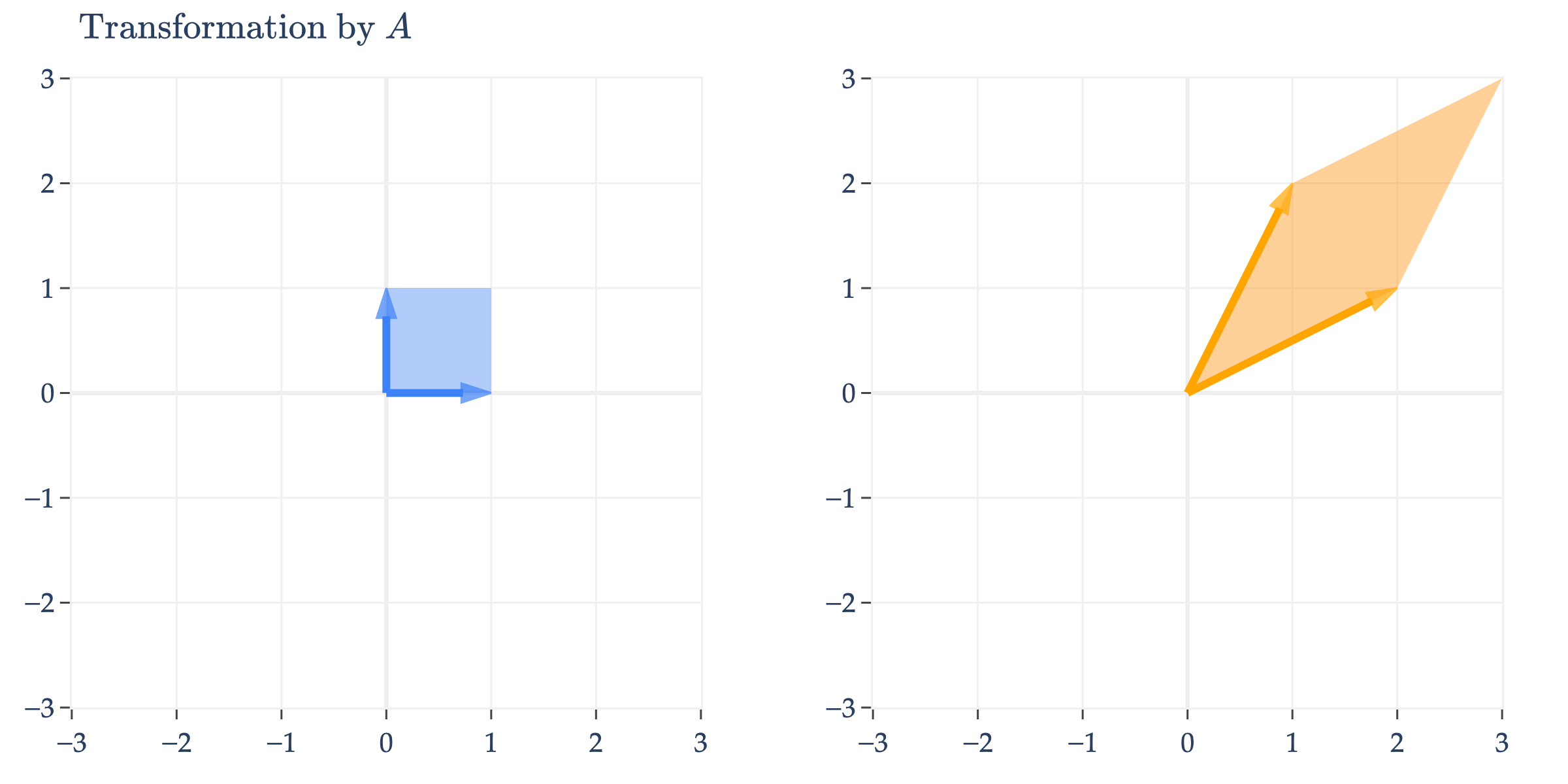
plot_unit_square_and_transform(B=A, name_B="A", show_labels=False, axis_range=[-3, 3], title=r'$$\text{Transformation by } A$$')

$A$ appears to perform an arbitrary transformation; it turns the unit square into a parallelogram, as we first saw in Chapter 2.9.

But, since $A$ is symmetric, it can be diagonalized by an orthogonal matrix, $A = Q \Lambda Q^T$ .

A = \begin{bmatrix} 1 & 2 \\ 2 & 1 \end{bmatrix}

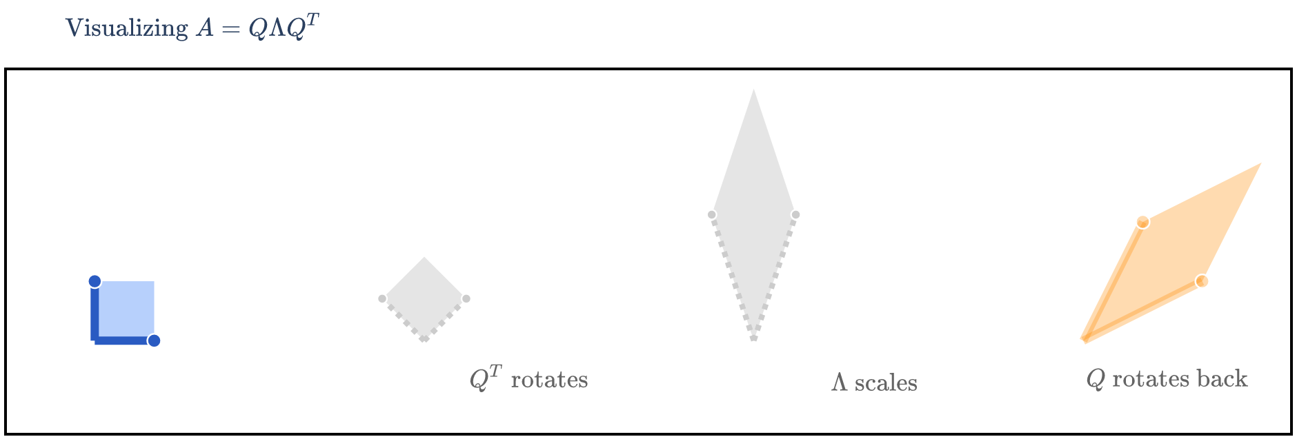
has eigenvalues $\lambda_1 = 3$ with eigenvector $\vec v_1 = \begin{bmatrix} 1 \\ 1 \end{bmatrix}$ and $\lambda_2 = -1$ with eigenvector $\vec v_2 = \begin{bmatrix} -1 \\ 1 \end{bmatrix}$ . But, the $\vec v_i$ ’s I’ve written aren’t unit vectors, which they need to be in order for $Q$ to be orthogonal. So, we normalize them to get $\vec q_1 = \begin{bmatrix} \frac{1}{\sqrt{2}} \\ \frac{1}{\sqrt{2}} \end{bmatrix}$ and $\vec q_2 = \begin{bmatrix} -\frac{1}{\sqrt{2}} \\ \frac{1}{\sqrt{2}} \end{bmatrix}$ . Placing these $\vec q_i$ ’s as columns of $Q$ , we get

Q = \begin{bmatrix} \frac{1}{\sqrt{2}} & -\frac{1}{\sqrt{2}} \\ \frac{1}{\sqrt{2}} & \frac{1}{\sqrt{2}} \end{bmatrix}

and so

A = Q \Lambda Q^T = \underbrace{\begin{bmatrix} \frac{1}{\sqrt{2}} & -\frac{1}{\sqrt{2}} \\ \frac{1}{\sqrt{2}} & \frac{1}{\sqrt{2}} \end{bmatrix}}_Q \underbrace{\begin{bmatrix} 3 & 0 \\ 0 & -1 \end{bmatrix}}_\Lambda \underbrace{\begin{bmatrix} \frac{1}{\sqrt{2}} & \frac{1}{\sqrt{2}} \\ -\frac{1}{\sqrt{2}} & \frac{1}{\sqrt{2}} \end{bmatrix}}_{Q^T}

We’re visualizing how $\vec x$ turns into $A \vec x$ , i.e. how $\vec x$ turns into $Q \Lambda Q^T \vec x$ . This means that we first need to consider the effect of $Q^T$ on $\vec x$ , then the effect of $\mathcal{\Lambda}$ on that result, and finally the effect of $Q$ on that result – that is, read the matrices from right to left.

import numpy as np
import plotly.graph_objects as go
from plotly.subplots import make_subplots

def plot_unit_square_diag_process(
    Q,
    Lambda,
    square_color="rgba(61,129,246,0.37)",  # blue for first subplot
    qt_color="rgba(255,140,0,0.31)",  # orange for last
    lqt_color=None,
    qlqt_color=None,
    sq_border_color="rgba(255,255,255,0)",
    show_arrows=True,
    xaxis_range=[-1.5, 3.5],
    yaxis_range=[1, 1],
    title="",
    return_fig=False,
    show_labels=True,
    names=None,  # list of 4 subplot titles
    vector_colors=None,
    vector_label_color="#222"
):
    # Colors for parallelograms
    fill_colors = [square_color, "rgba(180,180,180,0.35)", "rgba(180,180,180,0.35)", qt_color]

    # Arrows: 1st panel = blue, 2/3 = gray, 4th = orange
    BLUE = "#2a5bc2"
    ORANGE = qt_color if qt_color else "#ff8c00"
    GRAY = "#cccccc"
    arrow_colors = [BLUE, GRAY, GRAY, ORANGE]

    # Step labels for bottom right corner (not the first)
    step_labels = ["", r"$$Q^T \text{ rotates}$$", r"$$\Lambda \text{ scales}$$", r"$$Q \text{ rotates back}$$"]

    I = np.eye(2)
    M_list = [
        I,            # original unit square
        Q.T,          # first rotation/reflection
        Lambda @ Q.T, # scaling in new basis
        Q @ Lambda @ Q.T  # rotate back
    ]
    if not names:
        names = [
            r"Unit square",
            r"$Q^T$",
            r"$\Lambda Q^T$",
            r"$Q\Lambda Q^T$"
        ]

    square = np.array([
        [0, 0], [1, 0], [1, 1], [0, 1], [0, 0]
    ])
    u_x = np.array([1, 0])
    u_y = np.array([0, 1])

    fig = make_subplots(rows=1, cols=4,
                        subplot_titles=names,
                        horizontal_spacing=0.025)  # bring plots closer

    # Remove grid, ticks, numbers, and boxes completely
    axis_style = dict(
        showgrid=False,
        zeroline=False,
        showline=False,
        mirror=False,
        showticklabels=False,
        ticks="",
    )
    for j in range(4):
        fig.update_xaxes(range=xaxis_range, constrain="domain", **axis_style, row=1, col=j+1)
        fig.update_yaxes(range=yaxis_range, scaleanchor=f"x{j+1}", **axis_style, row=1, col=j+1)

    for j, M in enumerate(M_list):
        tr_square = (M @ square.T).T
        # Parallelogram
        fig.add_trace(
            go.Scatter(
                x=tr_square[:,0], y=tr_square[:,1],
                fill="toself",
                fillcolor=fill_colors[j],
                line=dict(color=sq_border_color, width=2 if j==0 else 1),
                name="Parallelogram",
                showlegend=False
            ),
            row=1, col=j+1)

        # Draw basis arrows for original and final panels, gray hidden arrows for intermediates
        if show_arrows:
            ux_t = M @ u_x
            uy_t = M @ u_y
            arrowwidth = 6 if j in [0,3] else 4
            arrowdot = 10 if j in [0,3] else 7
            vcolor = arrow_colors[j]
            # Draw for u_x, u_y
            for v, lbl in [(ux_t, r"$\vec u_x$"), (uy_t, r"$\vec u_y$")]:
                # Main arrow line
                fig.add_trace(go.Scatter(
                    x=[0, v[0]], y=[0, v[1]],
                    mode="lines",
                    line=dict(color=vcolor, width=arrowwidth, dash="solid" if j in [0,3] else "dot"),
                    showlegend=False,
                    hoverinfo="skip"
                ), row=1, col=j+1)
                # Arrowhead as dot
                fig.add_trace(go.Scatter(
                    x=[v[0]], y=[v[1]],
                    mode="markers",
                    marker=dict(size=arrowdot, color=vcolor, line=dict(width=1.2, color='white')),
                    showlegend=False,
                    hoverinfo="skip"
                ), row=1, col=j+1)
                # Only draw labels on blue and orange panels, or always if desired
                if show_labels and j in [0, 3]:
                    shift = 0.17 * (v / (np.linalg.norm(v)+1e-8))
                    fig.add_annotation(
                        text=lbl,
                        x=v[0] + shift[0], y=v[1] + shift[1],
                        font=dict(size=16, color=vector_label_color),
                        showarrow=False,
                        xanchor="left", yanchor="bottom",
                        row=1, col=j+1
                    )

        # Add step label in bottom right corner for panels 1,2,3 (not 0)
        if step_labels[j]:
            xr = xaxis_range if isinstance(xaxis_range[0], (int, float)) else xaxis_range[j]
            yr = yaxis_range if isinstance(yaxis_range[0], (int, float)) else yaxis_range[j]
            x_pos = xr[0] + 0.86*(xr[1] - xr[0])
            y_pos = yr[0] + 0.13*(yr[1] - yr[0]) - 2
            fig.add_annotation(
                text=step_labels[j],
                x=x_pos, y=y_pos,
                font=dict(size=20, color="rgba(100,100,100,0.85)", family="Palatino, serif"),
                showarrow=False,
                xanchor='right', yanchor='bottom',
                row=1, col=j+1
            )

    # --- Add box around the entire figure ---
    # We'll do this using a rectangle shape spanning the whole figure/plot coords.
    # Use xref/yref 'paper' so it covers all subplots, with margin fudge.
    fig.add_shape(
        type="rect",
        xref="paper",
        yref="paper",
        x0=0, y0=0,
        x1=1, y1=1,
        line=dict(color="black", width=2),
        fillcolor='rgba(0,0,0,0)',
        layer="above"
    )

    fig.update_layout(
        font=dict(family="Palatino, serif", size=16),
        plot_bgcolor="white",
        paper_bgcolor="white",
        # Whitespace reduced: smaller margins, smaller overall width
        margin=dict(l=4, r=4, t=50, b=10),
        width=940, height=325,
        title=title
    )
    if return_fig:
        return fig
    fig.show(renderer='png', scale=2)

# Example usage:
A = np.array([[1, 2], [2, 1]])
eigvals, eigvecs = np.linalg.eigh(A)
Q = eigvecs
Lambda = np.diag(eigvals)
plot_unit_square_diag_process(
    Q,
    Lambda,
    square_color="rgba(61,129,246,0.37)",
    qt_color="rgba(255,140,0,0.31)",
    # No need for lqt_color, qlqt_color; color ramp is used!
    sq_border_color="rgba(255, 255, 255, 0)",
    xaxis_range=[-1.5, 3.5],
    yaxis_range=[1, 2],
    title=r'$$\text{Visualizing } A = Q \Lambda Q^T$$',
    show_labels=False,
    names=[''] * 4
)

The Ellipse Perspective¶

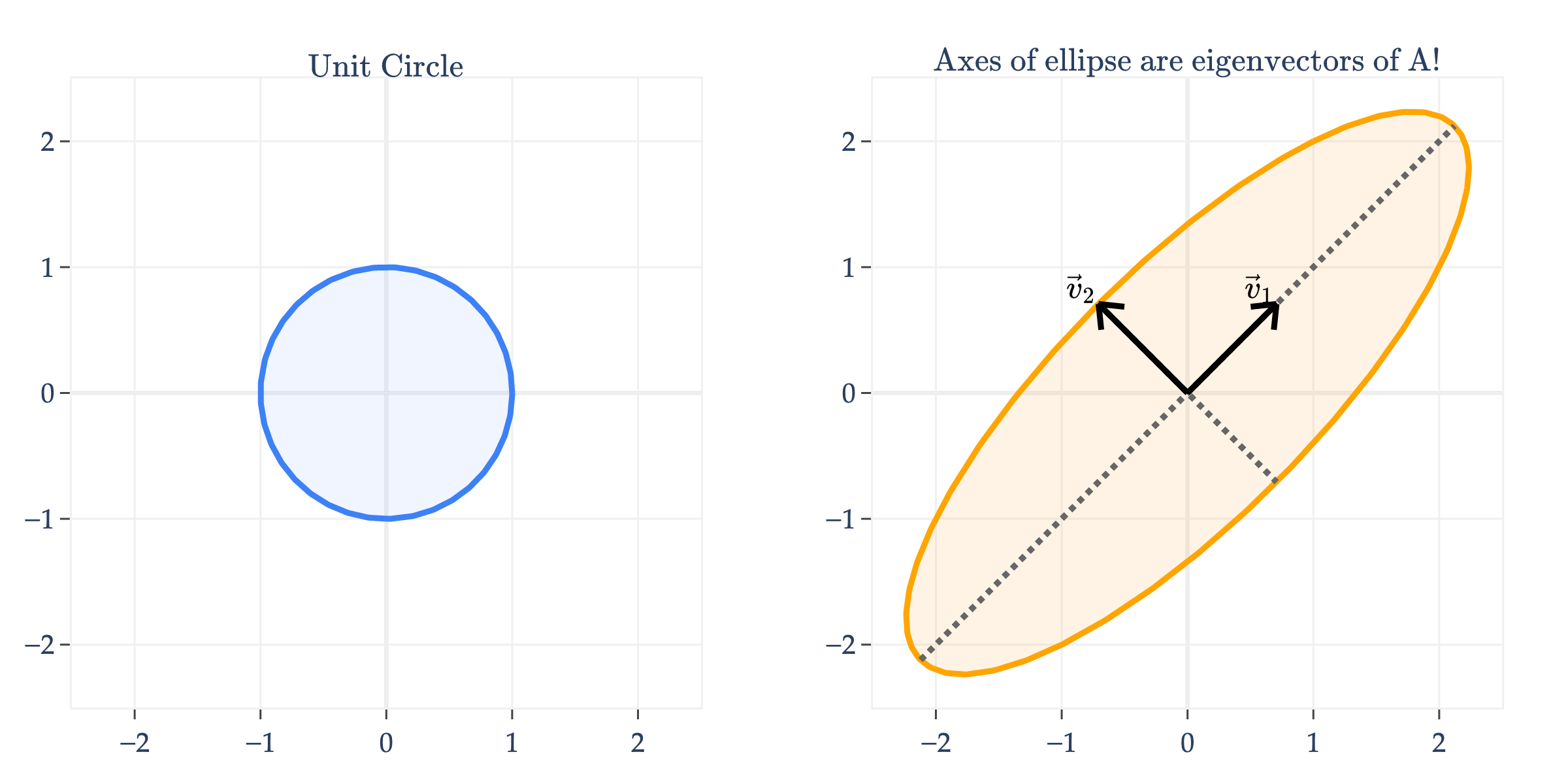
Another way of visualizing the linear transformation of a symmetric matrix is to consider its effect on the unit circle, not the unit square. Below, I’ll apply $A = \begin{bmatrix} 1 & 2 \\ 2 & 1 \end{bmatrix}$ to the unit circle.

import numpy as np
import plotly.graph_objects as go
from plotly.subplots import make_subplots

def plot_unit_circle_and_transform(S, name="Matrix", show_eig=True, return_fig=False):
    # Generate unit circle points
    theta = np.linspace(0, 2 * np.pi, 300)
    circle = np.vstack((np.cos(theta), np.sin(theta))).T
    # Transformed circle (ellipse)
    ellipse = (S @ circle.T).T

    # Compute real eigenvalues and eigenvectors (for drawing axes)
    try:
        eigvals, eigvecs = np.linalg.eig(S)
    except np.linalg.LinAlgError:
        eigvals, eigvecs = None, None
    # Only retain real-valued eigenvectors for the plot
    real_mask = np.abs(np.imag(eigvals)) < 1e-8
    real_eigvecs = np.real(eigvecs[:, real_mask])
    real_eigvals = np.real(eigvals[real_mask])
    # Normalize eigenvectors for plotting (unit)
    if real_eigvecs.shape[1] > 0:
        eigvec_norms = np.linalg.norm(real_eigvecs, axis=0)
        eigvecs_dir = real_eigvecs / eigvec_norms
    else:
        eigvecs_dir = np.zeros((2,0))

    # Set up figure
    fig = make_subplots(
        rows=1, cols=2,
        subplot_titles=(r"$$\text{Unit Circle}$$", fr"$$\text{{Axes of ellipse are eigenvectors of A!}}$$"),
        horizontal_spacing=0.08
    )

    # Common axis settings: [-2.5,2.5] for each
    axis_style = dict(
        showgrid=True,
        gridcolor="#f0f0f0",
        zeroline=False,
        showline=True,
        linecolor="#f0f0f0",
        mirror=True,
        ticks="outside",
        showticklabels=True,
        tickfont=dict(family="Palatino, serif", size=14),
    )
    # Apply axes settings to both; but you'll hide eigen-directions for left below
    for i in [1, 2]:
        fig.update_xaxes(
            range=[-2.5, 2.5],
            constrain="domain",
            dtick=1,
            **axis_style,
            row=1, col=i
        )
        fig.update_yaxes(
            range=[-2.5, 2.5],
            scaleanchor=f"x{i}",
            dtick=1,
            **axis_style,
            row=1, col=i
        )

    # Grid zero lines under all objects
    for i in [1,2]:
        fig.add_shape(
            type="line",
            x0=-2.5, x1=2.5, y0=0, y1=0,
            line=dict(color="rgba(170,170,170,0.25)", width=2, dash="solid"),
            row=1, col=i,
            layer="below"
        )
        fig.add_shape(
            type="line",
            x0=0, x1=0, y0=-2.5, y1=2.5,
            line=dict(color="rgba(170,170,170,0.25)", width=2, dash="solid"),
            row=1, col=i,
            layer="below"
        )

    # Left: unit circle (blue)
    fig.add_trace(
        go.Scatter(
            x=circle[:,0], y=circle[:,1],
            line=dict(color="#3d81f6", width=3),
            fill="toself",
            fillcolor="rgba(61,129,246,0.08)",
            name="Unit Circle",
            showlegend=False
        ),
        row=1, col=1
    )
    # Right: transformed circle (ellipse, orange)
    fig.add_trace(
        go.Scatter(
            x=ellipse[:,0], y=ellipse[:,1],
            line=dict(color="orange", width=3),
            fill="toself",
            fillcolor="rgba(255,140,0,0.10)",
            name="Transformed Circle",
            showlegend=False
        ),
        row=1, col=2
    )

    # Plot dotted lines for the (real) eigenvector directions
    # Only show eigenvector axes on right plot, and make them longer and #333 gray
    scale_left = 2.2  # keeps left here for compat but don't plot axes on left
    scale_right_1 = 3  # extend axes more on right plot
    scale_right_m1 = 1
    eig_axis_color = "#666"
    if show_eig and eigvecs_dir.shape[1] > 0:
        for i in range(eigvecs_dir.shape[1]):
            scale_right = scale_right_1 if i == 0 else scale_right_m1
            v = eigvecs_dir[:,i]
            # OMIT left side axes (ellipses axes, i.e. do NOT plot on left)
            # Show extended axes just on right (further and gray)
            for sign in [+1, -1]:
                # Only on right plot (ellipse)
                v_trans = S @ v
                v_trans_norm = np.linalg.norm(v_trans)
                if v_trans_norm > 1e-10:
                    v_trans_unit = v_trans / v_trans_norm
                    fig.add_trace(
                        go.Scatter(
                            x=[-scale_right * v_trans_unit[0], scale_right * v_trans_unit[0]],
                            y=[-scale_right * v_trans_unit[1], scale_right * v_trans_unit[1]],
                            mode="lines",
                            line=dict(color=eig_axis_color, width=3, dash="dot"),
                            name="Transformed Eigenvector",
                            hoverinfo="skip",
                            showlegend=False
                        ),
                        row=1, col=2
                    )

    # ---- Draw [1,1] and [-1,1] as black arrows on top of BOTH plots ----
    arrow_vectors = [np.array([1, 1]) / np.sqrt(2), np.array([-1, 1]) / np.sqrt(2)]
    arrow_colors = ['black', 'black']
    arrow_names = [r"$[1, 1]$", r"$[-1, 1]$"]
    arrow_length = 1  # scale for display

    for col in [2]:
        for idx, vec in enumerate(arrow_vectors):
            # Normalize for direction
            v = vec
            x0, y0 = 0, 0
            x1, y1 = arrow_length * v[0], arrow_length * v[1]
            fig.add_trace(
                go.Scatter(
                    x=[x0, x1],
                    y=[y0, y1],
                    mode="lines+markers",
                    line=dict(color=arrow_colors[idx], width=3),
                    marker=dict(size=1),
                    showlegend=False,
                    hoverinfo="skip"
                ),
                row=1, col=col
            )
            # Custom arrowhead using add_shape for nice head
            fig.add_shape(
                type="line",
                x0=x1-0.16*v[0]-0.13*v[1], y0=y1-0.16*v[1]+0.13*v[0], x1=x1, y1=y1,
                line=dict(color=arrow_colors[idx], width=3),
                row=1, col=col,
                layer="above"
            )
            fig.add_shape(
                type="line",
                x0=x1-0.16*v[0]+0.13*v[1], y0=y1-0.16*v[1]-0.13*v[0], x1=x1, y1=y1,
                line=dict(color=arrow_colors[idx], width=3),
                row=1, col=col,
                layer="above"
            )
            # Optionally add annotation at tip for column 1
            # Only show for one arrow to not clutter
            if col == 2:
                fig.add_annotation(
                    x=x1, y=y1,
                    text=fr"$$\vec v_{{{idx+1}}}$$",
                    showarrow=False,
                    font=dict(color='black', size=16),
                    row=1, col=col,
                    yanchor="bottom",
                    xanchor="right"
                )

    fig.update_layout(
        font=dict(family="Palatino, serif", size=16),
        plot_bgcolor="white",
        paper_bgcolor="white",
        margin=dict(l=20, r=20, t=40, b=20),
        width=800, height=400,
    )

    if return_fig:
        return fig
    fig.show(renderer='png', scale=3)

# Example usage:
A = np.array([[1, 2], [2, 1]])
plot_unit_circle_and_transform(A, name="A")

Notice that $A$ transformed the unit circle into an ellipse. What’s more, the axes of the ellipse are the eigenvector directions of $A$ !

Why is one axis longer than the other? As you might have guessed, the longer axis – the one in the direction of the eigenvector $\vec v_1 = \begin{bmatrix} 1 \\ 1 \end{bmatrix}$ – corresponds to the larger eigenvalue. Remember that $A$ has $\lambda_1 = 3$ and $\lambda_2 = -1$ , so the “up and to the right” axis is three times longer than the “down and to the right” axis, defined by $\vec v_2 = \begin{bmatrix} 1 \\ -1 \end{bmatrix}$ .

To see why this happens, consult the solutions to Lab 11, Activity 6b to try and derive it. It has to do with the expression $\sum_{i = 1}^n \lambda_i y_i^2$ ’s in that derivation. What are the $\lambda_i$ ’s and where did the $y_i$ ’s come from?

Positive Semidefinite Matrices¶

I will keep this section brief; this is mostly meant to be a reference for a specific definition that you used in Lab 11 and will use in Homework 10.

What does this have anything to do with the diagonalization of a matrix? We just spent a significant amount of time talking about the special properties of symmetric matrices, and positive semidefinite matrices are a subset of symmetric matrices, so the properties implied by the spectral theorem also apply to positive semidefinite matrices.

Positive semidefinite matrices appear in the context of minimizing quadratic forms, $f(\vec x) = \vec x^T A \vec x$ . You’ve toyed around with this in Lab 11, but also note that in Chapter 4.1 we saw the most important quadratic form of all: the mean-squared error!

\underbrace{R_\text{sq}(\vec w) = \frac{1}{n} \lVert \vec y - X \vec w \rVert^2}_{\text{this involves a quadratic form}}

If we know all of the eigenvalues of $A$ in $\vec x^T A \vec x$ are non-negative, then we know that $\vec x^T A \vec x \geq 0$ for all $\vec x$ , meaning that the quadratic form has a global minimum. This is why, as discussed in Lab 11, the quadratic form $\vec x^T A \vec x$ is convex if and only if $A$ is positive semidefinite.

The fact that having non-negative eigenvalues implies the first definition of positive semidefiniteness is not immediately obvious, but is exactly what we proved in Lab 11, Activity 6.

A positive definite matrix is one in which $\vec x^T A \vec x > 0$ for all $\vec x \neq \vec 0$ , i.e. where all eigenvalues are positive, not just non-negative (0 is no longer an option).

Key Takeaways¶

The eigenvalue decomposition of a matrix $A$ is a decomposition of the form
$A = V \Lambda V^{-1}$
where $V$ is a matrix containing the eigenvectors of $A$ as columns, and $\mathcal{\Lambda}$ is a diagonal matrix of eigenvalues in the same order. Only diagonalizable matrices can be decomposed in this way.
The algebraic multiplicity of an eigenvalue $\mathbf{\lambda}_i$ is the number of times $\mathbf{\lambda}_i$ appears as a root of the characteristic polynomial of $A$ .
The geometric multiplicity of $\mathbf{\lambda}$ is the dimension of the eigenspace of $\mathbf{\lambda}$ , i.e. $\text{dim}(\text{nullsp}(A - \lambda I))$ .
The $n \times n$ matrix is diagonalizable if and only if any of these equivalent conditions are true:
- $A$ has $n$ linearly independent eigenvectors.
- For every eigenvalue $\lambda_i$ , $\text{GM}(\lambda_i) = \text{AM}(\lambda_i)$ .
- $A$ has $n$ distinct eigenvalues.
When $A$ is diagonalizable, it has an eigenvalue decomposition, $A = V \Lambda V^{-1}$ .
If $A$ is a symmetric matrix, then the spectral theorem tells us that $A$ can be diagonalized by an orthogonal matrix $Q$ such that
$A = Q \Lambda Q^T$
and that all of $A$ ’s eigenvalues are guaranteed to be real.

What’s next? There’s the question of how any of this relates to real data. Real data comes in rectangular matrices, not square matrices. And even it were square, how does any of this enlighten us?