In Chapter 5 – which will last us the majority of the remainder of the semester – we’re going to introduce a new lens through which we can view the information stored in a matrix: through its eigenvalues and eigenvectors. As Gilbert Strang says in his book, eigenvalues and eigenvectors allow us to look into the “heart” of a matrix and see what it’s really doing.
Throughout this chapter, we’ll see how eigen-things can help us more deeply understand the topics we’ve already covered, like linear regression, the normal equations, gradient descent, and convexity.
The eigenvalues of the Hessian matrix (matrix of partial second derivatives) of a vector-to-scalar function will tell us whether or not the function is convex, i.e. they will give us a “second derivative test” for vector-to-scalar functions, which we haven’t yet seen.
Eigenvalues will explain why the matrix XTX+λI is always invertible, even if X’s columns aren’t linearly independent.
And eventually, in Chapter 5.3, we’ll use eigenvalues and eigenvectors to address the dimensionality reduction problem, first introduced in Chapter 1.1.
On top of all of that, eigenvalues and eigenvectors will unlock a new set of applications – those that involve some element of time. My favorite such example is Google’s PageRank algorithm. The algorithm, first published in 1998 by Sergey Brin and Larry Page (Google’s cofounders, the latter of whom is a Michigan alum), is used to rank pages on the internet based on their relative importance.
import networkx as nx
import numpy as np
import matplotlib.pyplot as plt
import seaborn as sns
from matplotlib_inline.backend_inline import set_matplotlib_formats

set_matplotlib_formats("svg")
sns.set_context("poster")
sns.set_style("whitegrid")
plt.rcParams["figure.figsize"] = (10, 5)

A = np.array([[0, 1 / 2, 1 / 2, 1 / 3],
              [1, 0, 0, 1 / 3],
              [0, 0, 0, 1 / 3],
              [0, 1 / 2, 1 / 2, 0]])

def plot_from_adjacency(adjacency_matrix, node_sizes=0.25):
    np.random.seed(25)
    plt.figure(figsize=(8, 5))
    G = nx.from_numpy_array(adjacency_matrix.T, create_using=nx.DiGraph)
    layout = nx.spring_layout(G)
    labels_dict={i: i+1 for i in range(adjacency_matrix.shape[0])}
    nx.draw(G, layout,
            node_size=15000 * node_sizes, labels=labels_dict, with_labels=True, font_color='white', font_weight='bold', font_size=15,
            connectionstyle='arc3, rad = 0.1')
    plt.show()

plot_from_adjacency(A)
Loading...
From the research paper linked above:
PageRank or PR(A) can be calculated using a simple iterative algorithm, and corresponds to the principal eigenvector of the normalized link matrix of the web.
We’ll make sense of the algorithm in Homework 10: just know that this is where we’re heading.
Before we get started, keep in mind that everything we’re about to introduce only applies to square matrices. This was also true when we first studied invertibility, and for the same reason: we should think of eigenvalues and eigenvectors as properties of a linear transformation from Rn to Rn (that is, from a vector space to itself), not between vector spaces of different dimensions. Rectangular matrices will have their moment in Chapter 5.3.
This definition is a bit hard to parse when you first look at it. But here’s the intuitive interpretation.
“Eigen” is a German word meaning “own”, as in “one’s own”. So, an eigenvector is a vector who still points in its own direction when transformed by A.
I’ve chosen the numbers in A to be small enough that we can roughly eyeball the eigenvectors. Here’s how I look at A:
First, notice that both rows of A sum to 3, meaning that
[1221][11]=[33]=3[11]
This tells me that [11] is an eigenvector of A with eigenvalue 3. But, [22] is also an eigenvector of A with the same eigenvalue, since
[1221][22]=[66]=3[22]
Indeed, if v is an eigenvector of A with eigenvalue λ, then so is cv for any non-zero scalar c. So really, eigenvectors define directions.
Additionally, noticing that there’d be some symmetry if I took the difference of the entries in each row of A, consider
[1221][−11]=[1−1]=−1[−11]
This tells me that [−11] is an eigenvector of A with eigenvalue -1.
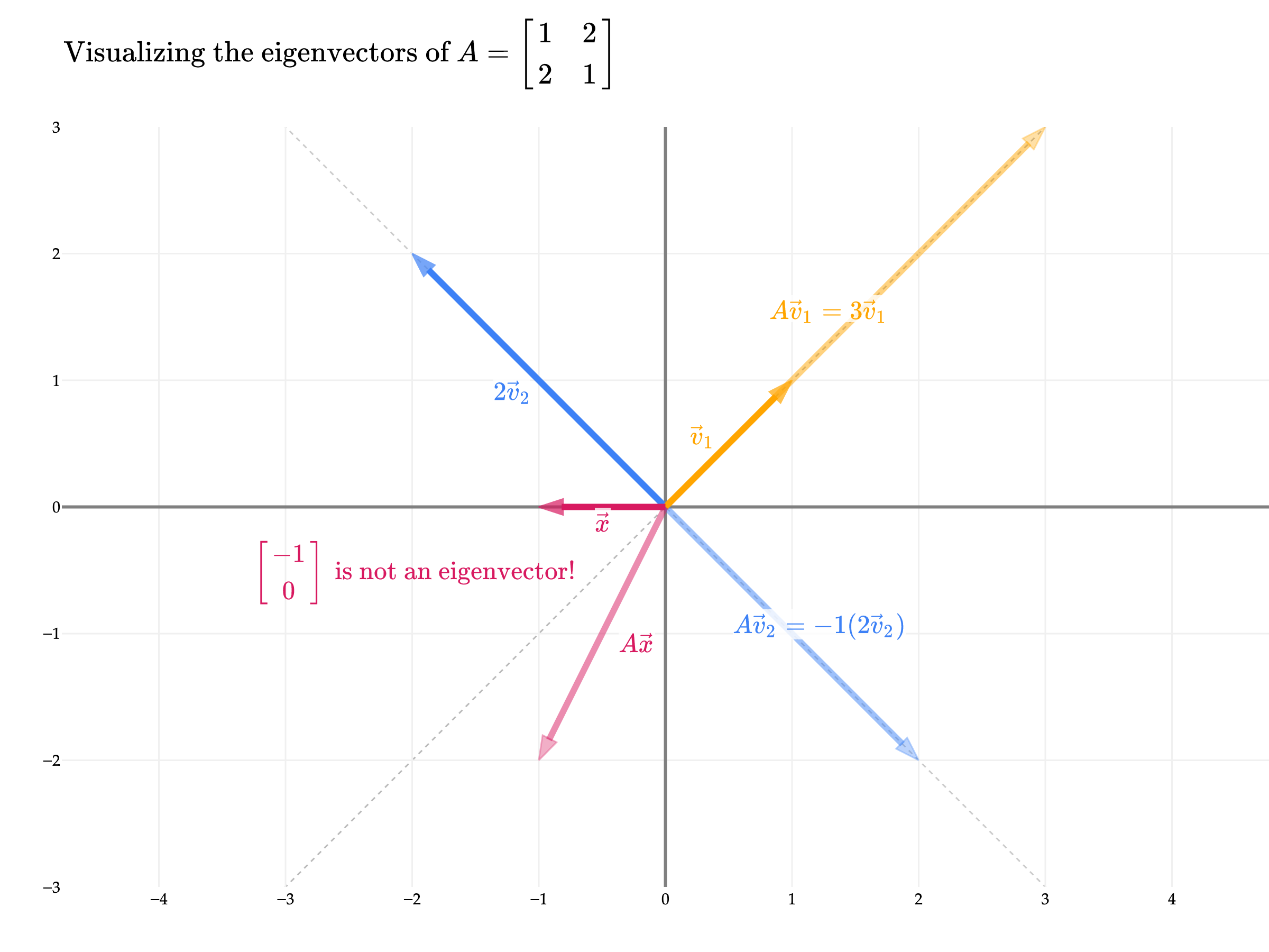
So, A=[1221] has two eigenvalues, 3 and -1, and two corresponding eigenvectors, [11] and [−11]. In general, an n×n matrix has n eigenvalues, but some of them may be the same, and some of them may not be real numbers. We’ll see how to systematically find these eigenvalues and eigenvectors in just a bit.
Visually, this means that v1=[11] lives on the same line as Av1, which is also the line that cv1 and A(cv1) live on (for any non-zero scalar c). And, v2=[−11] lives on the same line as Av2.
But, if a vector isn’t already on one of the two aforementioned lines – like x=[−10] – then it will change directions when multiplied by A, and it is not an eigenvector.
from utils import plot_vectors
import numpy as np

# Matrix
A = np.array([[1, 2], [2, 1]])

# Vectors
v1 = np.array([1, 1])      # eigenvector direction
v2 = np.array([-2, 2])    # same eigenvector direction, negative/scaled
x = -np.array([1, 0])
y = np.array([-2, -1])

Av1 = A @ v1
Av2 = A @ v2
Ax = A @ x
Ay = A @ y

# To set alpha=0.5 in hex, convert as follows:
# orange -> #FFA500   ===> with alpha=0.5: #80FFA500
# #3d81f6 -> with alpha=0.5: #803d81f6
# #d81a60 -> with alpha=0.5: #80d81a60
# #004d40 -> with alpha=0.5: #80004d40

vectors = [
    (tuple(v2), 'rgba(61,129,246,1.0)', r'$2\vec v_2$'),      # dimmed blue
    (tuple(Av2), 'rgba(61,129,246,0.5)', r'$A\vec v_2 = -1 (2\vec v_2)$'),    # full blue

    (tuple(v1), 'rgba(255,165,0,1.0)', r'$\vec v_1$'),       # dimmed orange
    (tuple(Av1), 'rgba(255,165,0,0.5)', r'$A\vec v_1 = 3 \vec v_1$'),     # full orange

    (tuple(x),  'rgba(216,26,96,1.0)', r'$\vec x$'),         # dimmed pink
    (tuple(Ax), 'rgba(216,26,96,0.5)', r'$A\vec x$'),        # full pink

]

# Prepare faint lines along the two eigenvector directions: [1,1] and [-1,1]
line_length = 6
eig1_dir = np.array([1, 1]) / np.linalg.norm([1, 1])
eig2_dir = np.array([-1, 1]) / np.linalg.norm([-1, 1])

eig1_line1 = eig1_dir * line_length
eig1_line2 = -eig1_dir * line_length
eig2_line1 = eig2_dir * line_length
eig2_line2 = -eig2_dir * line_length

background_lines = [
    ((eig1_line1[0], eig1_line1[1]), (eig1_line2[0], eig1_line2[1]), "#bbbbbb", "dot"),
    ((eig2_line1[0], eig2_line1[1]), (eig2_line2[0], eig2_line2[1]), "#cccccc", "dot"),
]

fig = plot_vectors(
    vectors,
    # background_lines=background_lines,
    vdeltay=0.1
)

# Add dotted lines in the eigenvector directions
for line in background_lines:
    (x0, y0), (x1, y1), color, dash = line
    fig.add_shape(
        type="line",
        x0=x0, y0=y0, x1=x1, y1=y1,
        line=dict(color=color, width=1, dash="dot"),
        layer="below"
    )

fig.update_layout(
    xaxis=dict(range=[-3, 3], dtick=1),
    yaxis=dict(scaleanchor="x", range=[-3, 3], dtick=1),
    title=r"$$\text{Visualizing the eigenvectors of } A = \begin{bmatrix} 1 & 2 \\ 2 & 1 \end{bmatrix}$$",
    margin=dict(l=0, r=0, t=80, b=0)
)

# Annotate [-1, 0] is not an eigenvector at the bottom left in #d81a60
fig.add_annotation(
    x=-2, y=-0.5,
    text=r"$$\begin{bmatrix} -1 \\ 0 \end{bmatrix} \text{ is not an eigenvector!}$$",
    font=dict(color="#d81a60", size=16),
    showarrow=False,
    align="left"
)

fig.show(scale=3, renderer='png')
Just to be 100% clear, I’ve used v2 instead of v2 above just to illustrate the fact that eigenvectors are only defined up to a scalar multiple; 2v2 is just as good as an eigenvector as v2 is, and both correspond to the same eigenvalue, λ=1.
You might notice that the two eigenvectors of A corresponding to the two different eigenvalues are orthogonal in the example above. This is not true in general for any 2×2 matrix, but there’s a specific reason it’s true for A: it’s symmetric. I’ll elaborate more on this idea in Chapter 5.3, but for now, just remember that symmetric matrices have orthogonal eigenvectors.
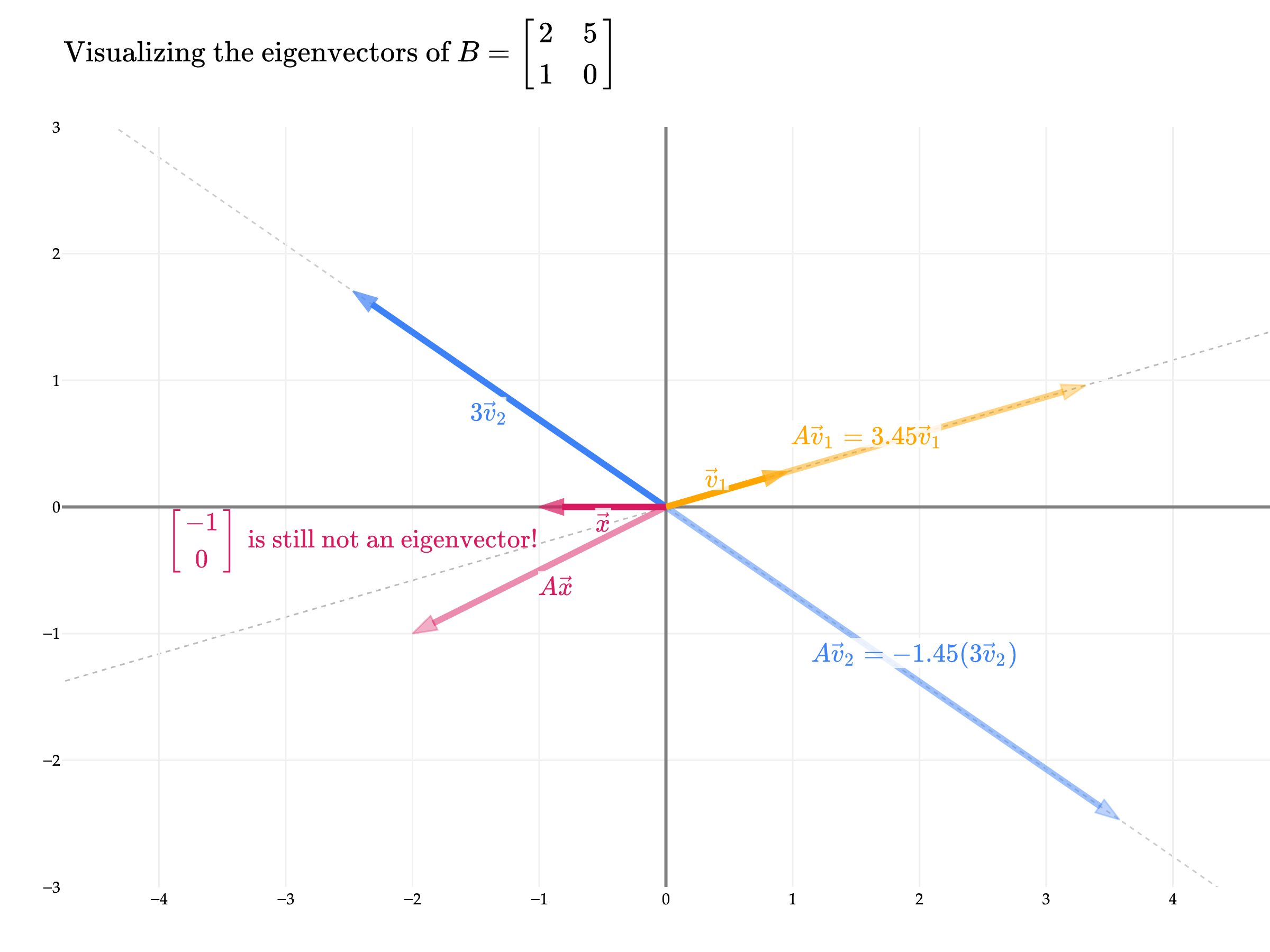
Its eigenvalues and eigenvectors aren’t particularly nice, and since we don’t yet have a way to find them by hand, now is as good as a time as any to use numpy:
eigvecs is a matrix where each column is an eigenvector of B. For now, call this matrix P. Below, I calculate PTP, which contains the dot products of all pairs of eigenvectors of B. The diagonal of this matrix contains the dot products of each eigenvector with itself; since these are 1, this tells us that the returned eigenvectors are unit vectors. This was a design decision by the implementors of np.linalg.eig – remember that we can scale an eigenvector by any non-zero scalar and it is still an eigenvector. The off-diagonal entries of -0.632 tell us that the two eigenvectors are not orthogonal.
eigvecs.T @ eigvecs
array([[ 1.        , -0.63245553],
       [-0.63245553,  1.        ]])
Let’s take a look at the directions of the eigenvectors for B.
from utils import plot_vectors
import numpy as np

# Matrix
A = np.array([[2, 5], [1, 0]])

# Find eigenvalues and eigenvectors
eigvals, eigvecs = np.linalg.eig(A)

# Pick v1 to be the *unit* eigenvector for the first eigenvalue (use eigvecs[:,0])
v1_unit = eigvecs[:, 0]# / np.linalg.norm(eigvecs[:, 0])
v1 = v1_unit

# Pick v2 to be *three times* the unit eigenvector for the second eigenvalue (eigvecs[:,1])
v2 = 3 * eigvecs[:, 1]# / np.linalg.norm(eigvecs[:, 1])

x = -np.array([1, 0])

Av1 = A @ v1
Av2 = A @ v2
Ax = A @ x

# To set alpha=0.5 in hex, convert as follows:
# orange -> #FFA500   ===> with alpha=0.5: #80FFA500
# #3d81f6 -> with alpha=0.5: #803d81f6
# #d81a60 -> with alpha=0.5: #80d81a60
# #004d40 -> with alpha=0.5: #80004d40

vectors = [
    (tuple(v2), 'rgba(61,129,246,1.0)', r'$3\vec v_2$'),      # dimmed blue (same as A example but 3*v2)
    (tuple(Av2), 'rgba(61,129,246,0.5)', r'$A\vec v_2 = %.2f (3\vec v_2)$' % eigvals[1]),    # full blue, faded
    (tuple(v1), 'rgba(255,165,0,1.0)', r'$\vec v_1$'),       # dimmed orange (matches prior coloring)
    (tuple(Av1), 'rgba(255,165,0,0.5)', r'$A\vec v_1 = %.2f \vec v_1$' % eigvals[0]),     # full orange, faded
    (tuple(x),  'rgba(216,26,96,1.0)', r'$\vec x$'),         # dimmed pink
    (tuple(Ax), 'rgba(216,26,96,0.5)', r'$A\vec x$'),        # full pink, faded
]

# Prepare faint lines along the two eigenvector directions (use actual directions from eigvecs)
line_length = 6
eig1_dir = v1_unit
eig2_dir = eigvecs[:, 1] / np.linalg.norm(eigvecs[:, 1])

eig1_line1 = eig1_dir * line_length
eig1_line2 = -eig1_dir * line_length
eig2_line1 = eig2_dir * line_length
eig2_line2 = -eig2_dir * line_length

background_lines = [
    ((eig1_line1[0], eig1_line1[1]), (eig1_line2[0], eig1_line2[1]), "#bbbbbb", "dot"),
    ((eig2_line1[0], eig2_line1[1]), (eig2_line2[0], eig2_line2[1]), "#cccccc", "dot"),
]

fig = plot_vectors(
    vectors,
    # background_lines=background_lines,
    vdeltay=0.1
)

# Add dotted lines in the eigenvector directions
for line in background_lines:
    (x0, y0), (x1, y1), color, dash = line
    fig.add_shape(
        type="line",
        x0=x0, y0=y0, x1=x1, y1=y1,
        line=dict(color=color, width=1, dash="dot"),
        layer="below"
    )

fig.update_layout(
    xaxis=dict(range=[-3, 3], dtick=1),
    yaxis=dict(scaleanchor="x", range=[-3, 3], dtick=1),
    title=r"$$\text{Visualizing the eigenvectors of } B = \begin{bmatrix} 2 & 5 \\ 1 & 0 \end{bmatrix}$$",
    margin=dict(l=0, r=0, t=80, b=0)
#
)

# Annotate [-1, 0] is not an eigenvector at the bottom left in #d81a60
fig.add_annotation(
    x=-2.5, y=-0.25,
    text=r"$$\begin{bmatrix} -1 \\ 0 \end{bmatrix} \text{ is still not an eigenvector!}$$",
    font=dict(color="#d81a60", size=16),
    showarrow=False,
    align="left"
)

fig.show(scale=3, renderer='png')
While the eigenvectors of B are not orthogonal, they are still linearly independent and span all of R2. This was also the case in the A example above. The fact that the eigenvectors of an n×n matrix are linearly independent and span all of Rn is also not guaranteed to be true, though it’s a desirable property. The class of matrices that have this property are called diagonalizable, which are the focus of Chapter 5.3.
Let’s consider a few more examples, each of which is meant to highlight a different key property of eigenvalues and eigenvectors.
Let A=[1221] be the matrix from the first example above. What are the eigenvalues and eigenvectors of A2? Find them manually. You should notice the property below.
Solution
A2=[1221][1221]=[5445]
Similar to the original example, A2’s rows both sum to the same number, 9, meaning that
[5445][11]=[99]=9[11]
We can do the same thing with A2[1−1]:
A2[1−1]=[1−1]=1[1−1]
So the eigenvalues of A2 are 9 and 1, and their respective eigenvectors are [11] and [1−1].
But, these are the same two eigenvectors that A has, and the corresponding eigenvalues are the squares of A’s eigenvalues, since 32=9 and (−1)2=1. Is this true more generally? Yes!
If λ is an eigenvalue of A with eigenvector v, then λk is an eigenvalue of Ak with the same eigenvector v. (Click to see the proof.)
A quick proof: suppose Av=λv. Then,
A2v=A(Av)=A(λv)=λ(Av)=λ2v
This logic can be extended to A3, then A4, and so on. (If you are familiar with induction from EECS 203, you can think of this as an inductive proof.)
Note that the converse of this statement is not necessarily true, meaning it’s possible for A2 to have an eigenvector that is not an eigenvector of A. For example, if A corresponds to a rotation by 90º degrees (or 2π radians), then A2 corresponds to a rotation by 180º degrees (or π radians). No vector lies on the same line after rotation by 90º degrees, but all vectors lie on the same line after rotation by 180º degrees. So, in this example, A2 has plenty of eigenvectors that A does not have.
Let A=[13412]. Notice that rank(A)=1. A has an eigenvalue of 13 with eigenvector [13] – verify that this is the case. Does it have another eigenvalue? What is the corresponding eigenvector?
Solution
Since rank(A)=1, A has a non-trivial null space, and any vector in the null space will get sent to 0 times itself when multiplied by A. Since 4⋅column 1=column 2, the null space of A is spanned by the vector [4−1]. So,
A[4−1]=[13412][4−1]=[00]=0[4−3]
0 can’t be an eigenvector, but 0 is a perfectly good eigenvalue.
Our intuition tells us that A should have another eigenvalue, since it’s a 2×2 matrix. It happens to be 13, corresponding to the eigenvector [13]. In the section titled “The Characteristic Polynomial”, we’ll see how to find this eigenvalue-eigenvector pair without guesswork.
0 is an eigenvalue of A if and only if A is not invertible. (Click to see more details.)
If A is invertible, then the only solution to Av=0v=0 is the trivial solution where v is the zero vector itself. But, we defined eigenvectors to be non-zero vectors. So, 0 can’t be an eigenvalue of an invertible matrix. If A is not invertible, then A has a non-trivial null space, and any non-zero vector in the null space is an eigenvector corresponding to the eigenvalue 0.
What are the eigenvalues and eigenvectors of I=[1001]?
Solution
The identity matrix multiplied by any vector v returns that same vector back, meaning that all vectors in R2 are eigenvectors of I, all with eigenvalue 1.
This is the first example we’ve seen so far where there exist multiple “lines” or “directions” of eigenvectors for a single eigenvalue. The vectors [23] and [−14] are both eigenvectors of I with eigenvalue 1 but they don’t lie on the same line. We will study this idea – of having multiple eigenvector directions for a single eigenvalue – more precisely in Chapter 5.3.
So far, we’ve found the eigenvalues and eigenvectors of a matrix by eyeballing them or reasoning about them geometrically, but this is not a sustainable strategy. Let’s develop a more systematic approach.
We’re looking for combinations of scalars, λ, and vectors, v, such that
Av=λv
In some ways, we’re trying to “solve” for λ and v given A. Let’s experiment a little:
Av=λvAv−λv=0(A−λI)v=0
What the above says is that if v is an eigenvector of A with eigenvalue λ, then v is in the null space of A−λI. But, since eigenvectors can’t be the zero vector, this means that A−λI is not invertible, since it has a non-trivial null space!
Thinking back to Chapter 2.9, we know that there are several equivalent ways to check if a matrix is not invertible. Perhaps the most computational approach is to compute its determinant; if a (square) matrix’s determinant is 0, then it is not invertible, otherwise it is.
So, since A−λI is not invertible, its determinant must be 0!
Av=λv⟹det(A−λI)=0
(We won’t always use the symbol p(λ), I just introduced it above to make it clear that det(A−λI) is a polynomial function of λ.)
Let’s revisit our example A=[1221].
The matrix A−λI is
A−λI=[1221]−λ[1001]=[1−λ221−λ]
Note that A−λI involves subtracting λ from the diagonal elements of A, and leaving all other elements unchanged.
The determinant of A−λI is
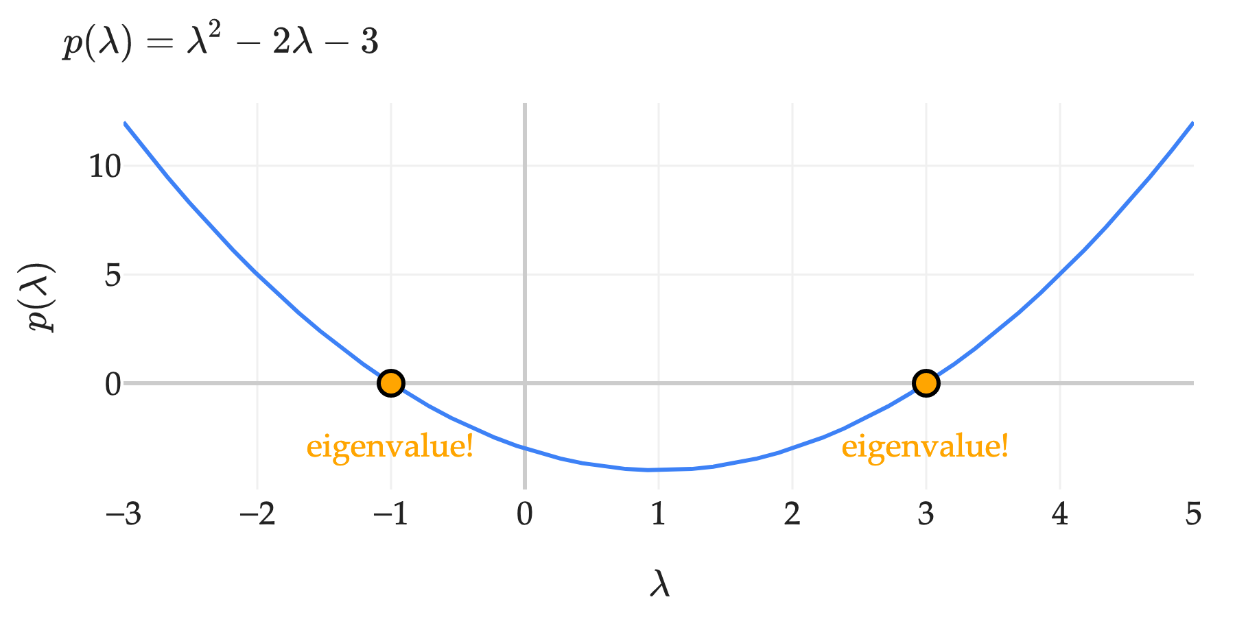
det(A−λI)=(1−λ)(1−λ)−2⋅2=λ2−2λ+1−4=p(λ)λ2−2λ−3
The eigenvalues of A are the values of λ where λ2−2λ−3=0.
(In general, we’re not going to plot the characteristic polynomial each time, but I think it’s useful to see once or twice to give the idea some context.)
By factoring, I can write this equation as
(λ+1)(λ−3)=0
which tells me that the eigenvalues of A are λ1=−1 and λ2=3. If this equation weren’t factorable, I’d need to use the quadratic formula to find the eigenvalues. For now, there’s no particular “ordering” to the eigenvalues, i.e. I could have said λ1=3 and λ2=−1; all that matters is that I stay consistent throughout a particular example.
Once we find the eigenvalues by solving p(λ)=0, we can find the eigenvectors by solving (A−λI)v=0 for each eigenvalue.
For λ1=−1, we’re looking for vectors v such that Av=−1v, i.e. if v=[ab], then
[1221][ab]=[−a−b]
(I’m using a and b instead of v1 and v2 because I’ll refer to the vectors v1 and v2 in just a moment.) As a system of equations, this says
a+2b2a+b=−a=−b
The first and second equations both tell us that b=−a. Remember, we’d expect there to be infinitely many solutions to this system, since any scalar multiple of an eigenvector is still an eigenvector. So, the “simple” solution is v1=[1−1], but [2−2], [3−3], etc. are also solutions.
For λ2=3, let me introduce another way of finding the corresponding eigenvector. There’s nothing wrong with the system of equations approach, but it’s useful to have multiple techniques for solving problems in our toolkit. λ2=3 tells us that Av=3v, or equivalently, (A−3I)v=0. So, the eigenvector we’re looking for is in the null space of A−3I.
A−3I=[1−3221−3]=[−222−2]
Here, we notice that both rows of A−3I sum to 0, meaning that
So our eigenvalues are λ1=2 and λ2=5. Next, let’s find eigenvectors for them. As I did in the first example, I’ll show two different techniques for finding eigenvectors.
For λ1=2, we’re looking for a vector v=[ab] such that Av=2v:
Av[3214][ab]3a+b2a+4b=2v=[2a2b]=2a=2b
As expected, there are infinitely many choices for a and b (since both equations tell us that b=−a), and the resulting eigenvectors v all lie on the same line. So, if we let a=1, then we have that v1=[1−1] is an eigenvector for λ1.
For λ2=5, I’ll try the null space approach, just to illustrate it once more. Again, I’m looking for a vector v such that Av=5v, or equivalently, (A−5I)v=0.
A−5I=[3−5214−5]=[−221−1]
The vector v2=[12] is orthogonal to both rows of A−5I, meaning (A−5I)[12]=[00]. So, v2=[12] is an eigenvector for λ2=5, though again any non-zero scalar multiple of [12] will also be an eigenvector for λ2=5.
So, A has eigenvalues λ1=2 and λ2=5, and corresponding eigenvectors v1=[1−1] and v2=[12].
Find the eigenvalues and eigenvectors of A=[300−4]. What do you notice about the eigenvalues? The eigenvectors?
Solution
The key is to notice that for diagonal matrices – that is, matrices where all the entries off the diagonal are 0 – the eigenvalues are simply the entries on the diagonal.
A−λIdet(A−λI)=[3−λ00−4−λ]=(3−λ)(−4−λ)
The eigenvalues λ1=3 and λ2=−4 are the same as the values on the diagonal! The corresponding eigenvectors are v1=[10] and v2=[01]. Just to illustrate one of those cases out,
Av2=[300−4][01]=[0−4]=−4[01]
The fact that eigenvalues and eigenvectors are so easy to find for diagonal matrices, coupled with the fact that diagonal matrices are really easy to compute powers of (e.g. A2 is just the diagonal matrix with each entry squared), makes them very useful in practice.
Find two different2×2 matrices who have the characteristic polynomial
p(λ)=λ2−4λ+3
Solution
Recall that for a 2×2 matrix A=[acbd]:
p(λ)=det(A−λI)=∣∣a−λcbd−λ∣∣=(a−λ)(d−λ)−bc
A simple approach to this problem is to find 2 diagonal matrices D=[a00d] and D′=[d00a]. That way, all we have to do is factor p(λ) into the form (a−λ)(d−λ):
λ2−4λ+3=(3−λ)(1−λ)
So, our two different matrices are D=[3001] and D′=[1003].
There exist non-diagonal matrices with the same characteristic polynomial, too. For instance,
[2112]
also has eigenvalues of 1 and 3, and its characteristic polynomial is also p(λ)=λ2−4λ+3.
So, the eigenvalues are the values along the diagonal: λ1=3, λ2=1, and λ3=2. This is a convenient property of triangular matrices (which is why I’ve planted this example here). Next, let’s find their eigenvectors.
For λ1=3, I’ll do it the null space way: I’m looking for a vector in the null space of A−3I. (I say “the null space way” but it’s really just a different way of writing the system of equations approach, and one that can sometimes be easier to eyeball.)
A−3I=⎣⎡0003−2005−1⎦⎤
The zeros in the first column tell me that (A−3I)⎣⎡100⎦⎤=⎣⎡000⎦⎤, so v1=⎣⎡100⎦⎤ is an eigenvector for λ1=3. Because I have three unique eigenvalues and my matrix is 3×3, I know that this is the only possible eigenvector direction for λ1=3; in Chapter 5.3, we’ll run into situations where the null space of A−3I (for instance) is spanned by more than one vector, but that’s not the case here.
For λ2=1, I’ll do it the system of equations way: I’m looking for a vector v=⎣⎡abc⎦⎤ such that Av=1v.
Once again, there are infinitely many solutions to this system, which we’d expect since there’s a whole line of eigenvectors.
The third equation above tells us that c=0.
Substituting that into the second equation, we have that b+5⋅0=b, i.e. b=b, so let’s treat b as a free variable for now.
The first equation above tells us that 3a+3b=a, i.e. a=−23b.
So, any vector of the form ⎣⎡−23bb0⎦⎤ is an eigenvector for λ2=1. But we just need to find one, so let’s take b=2, which gives us v2=⎣⎡−320⎦⎤.
Finally, for λ3=2, I’ll do it the null space way.
A−2I=⎣⎡3−20031−20052−2⎦⎤=⎣⎡1003−10050⎦⎤
I’m looking for a vector v3=⎣⎡abc⎦⎤ in the null space of A−2I, i.e. a vector whose dot product with each row of A−2I is 0. The last row of A−2I is all zeros, so I can focus my attention on the first two rows. If the first two components of v3 are -3 and 1, then the dot product of v3 with the first row of A−2I is (1)(−3)+(3)(1)=0, which is what I want.
Then, its dot product with the second row is (0)(−3)+(−1)(1)+(5)(c)=−1+5c, where c is the last component of v3. For −1+5c=0, we need c=51. So, one vector in the null space of A−2I – which is an eigenvector for λ3=2 – is v3=⎣⎡−3151⎦⎤. To clean the numbers up a bit, I’ll scale this vector by 5, which gives us v3=⎣⎡−1551⎦⎤.
So, our eigenvectors for λ1=3, λ2=1, and λ3=2 are v1=⎣⎡100⎦⎤, v2=⎣⎡−320⎦⎤, and v3=⎣⎡−1551⎦⎤.
# When in doubt, check with numpy!
np.linalg.eig(
    np.array([
        [2, 0, 0],
        [-1, 5, 0],
        [4, 3, -7]
    ])
)
The characteristic polynomial of an n×n matrix is a polynomial of degree n. A fact from algebra is that a polynomial of degree n has exactly n roots. The intuitive way of thinking about this is that degree n polynomials can have at most n−1 “bends” (a line can’t bend, a quadratic can bend once, a cubic can bend twice, etc.), and each time it bends, it can change directions to cross the x-axis again.
The issue is that some of these roots may be repeated, and some may be complex numbers, meaning that they don’t actually cross the x-axis in the standard xy-plane (or in our case, the λ-axis and λ,p(λ)-plane).
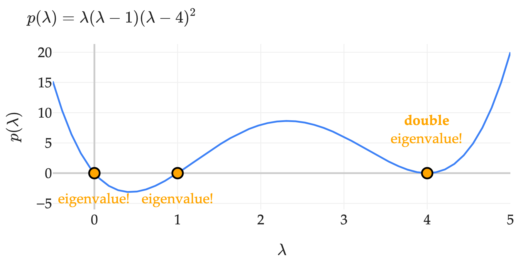
For example, the matrix A=⎣⎡4000010000000004⎦⎤ is diagonal, meaning its easy to read off its characteristic polynomial:
This characteristic polynomial has a double root at λ=4, a single root at λ=1, and a single root at λ=0. This A has 3 distinct eigenvalues, but one of them, λ=2, is repeated, and has an algebraic multiplicity of 2.
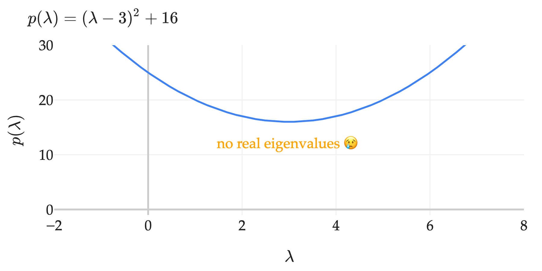
As another example, the matrix A=[34−43] has the characteristic polynomial
p(λ)=∣∣3−λ4−43−λ∣∣=(λ−3)2+16
I can expand this out to get λ2−6λ+25, but in a case like this I think the above form is more telling. Visually, p(λ) here is a parabola that sits entirely above the λ-axis, meaning it has no real roots, so A has no real eigenvalues.
where θ=cos−1(53). This matrix rotates vectors by θ radians counterclockwise, which means that no real-valued vector will remain in the same direction after being multiplied by A. In the 2×2 case, the only way to get a real-valued eigenvalue out of a rotation matrix is if the matrix rotates by an integer multiple of π radians (180 degrees), which either corresponds to reflecting/negating the vector (like in [−100−1]) or returning back the same vector itself (like in [1001], the identity matrix, which can be thought of as a rotation by 2π).
The solutions to p(λ)=(λ−3)2+16=0 are the complex numbers λ=3+4i and λ=3−4i, again where i is the imaginary unit, defined by i2=−1. The corresponding eigenvectors are complex too, and we won’t worry about finding them. (If you’re familiar with complex numbers, you might recognize these eigenvalues as 5eiθ and 5e−iθ, where θ=cos−1(53). This comes from Euler’s formula, eiθ=cosθ+isinθ.)
The coefficient on λ is −(a+d), which is the negative of the sum of the diagonal entries of A. A term often used to refer to the sum of the diagonal entries of a matrix is its trace, trace(A). And, the constant term of p(λ) above is just det(A)! For 2×2 matrices, this says that the characteristic polynomial is of the form
p(λ)=λ2−trace(A)λ+det(A)
For example, consider A=[3719]. The fact above says that A’s characteristic polynomial is
p(λ)=λ2−(3+9)λ+(3⋅9−1⋅7)=λ2−12λ+20
which, with enough practice, is a calculation you might be able to do in your head. But, this gives way to a more general fact, that is true for any n×n matrix.
Example 1: A=[3719]'s eigenvalues add up to 3+9=12 and multiply to det(A)=3⋅9−1⋅7=20. This gives me a quick way of figuring out that A’s eigenvalues are 10 and 2.
Example 2: A=⎣⎡0.50.400.50.30.500.30.5⎦⎤ has an eigenvalue of 1, corresponding to the eigenvector ⎣⎡111⎦⎤, since the sum of each row of A is 1. Let λ2 and λ3 be the other two eigenvalues. The trace fact tells me that
In other words, the other two eigenvalues sum to 0.3 and multiply to -0.1. This sounds like a job for 0.5 and -0.2, which are indeed the other two eigenvalues of A (other than 1).
Example 3: A=[1224] has a determinant of 1⋅4−2⋅2=0, which means that its eigenvalues multiply to 0, which is another reminder that A has an eigenvalue of 0. The trace fact tells me that the other eigenvalue λ2 must satisfy 1+4=0+λ2, so λ2=5.
λ is an eigenvalue of A, corresponding to the eigenvector v, if
Av=λv
The English interpretation of this is that v is an eigenvector of A if, when multiplied by A, v still points in the same direction, and is just stretched by a factor of λ.
An n×n matrix A has exactly n eigenvalues. Some of these may be complex, and some of these may be repeated, but all of them are roots to the characteristic polynomial of A,
p(λ)=det(A−λI)
A quick way to check if you’ve found the right eigenvalues is that
The product of the eigenvalues of A is equal to det(A), i.e. λ1λ2⋯λn=det(A).
The sum of the eigenvalues of A is equal to the trace of A, which is the sum of the diagonal elements of A.
0 is an eigenvalue of A if and only if A is not invertible.
If λ is an eigenvalue of A with eigenvector v, then λk is an eigenvalue of Ak with the same eigenvector v.