4.4. Lines, Planes, Hyperplanes, and the Cross Product
Think of this section as a brief detour from the main storyline of the course. Here, I’ll cover how to describe lines, planes, and hyperplanes in Rn, and how they relate to our understanding of spans and subspaces from earlier in this chapter.
We’re very familiar with lines in R2. The line y=2x+3, in R2, is the set of all (x,y) coordinates that satisfy the equation y=2x+3.
The line y=2x+3 is in slope-intercept form, which more generally looks like y=w0+w1x. Sometimes, we may write lines in standard form, like 2x−y+3=0, or more generally, ax+by+c=0.
Let’s kick things up a notch and consider lines in R3. What is the equation of theline below?
from utils import plot_vectors
import numpy as np
import plotly.graph_objects as go

v = (2, -1, 3)

# Create the line spanned by v (all scalar multiples)
t = np.linspace(-2, 2, 100)
line_x = t * v[0]
line_y = t * v[1]
line_z = t * v[2]

fig = plot_vectors([((0, 0, 0), "#3d81f6", r"")], show_axis_labels=True, vdeltax=0.1)

# Add the line spanned by v to the 3D plot
fig.add_trace(
    go.Scatter3d(
        x=line_x,
        y=line_y,
        z=line_z,
        mode="lines",
        line=dict(color="rgba(0,77,64,0.6)", width=5),
        showlegend=False,
        hoverinfo="skip"
    )
)

# Draw small points at (0, 0, 0) and the tip of v
fig.add_trace(
    go.Scatter3d(
        x=[0, v[0]],
        y=[0, v[1]],
        z=[0, v[2]],
        mode="markers",
        marker=dict(size=4, color=["#222", "#222"]),
        showlegend=False,
        hoverinfo="skip"
    )
)

# Add annotations next to the two points: (0,0,0) and (2,-1,3)
fig.add_trace(
    go.Scatter3d(
        x=[0],
        y=[0],
        z=[0],
        mode="text",
        text=["(0, 0, 0)"],
        textposition="top right",
        showlegend=False,
        hoverinfo="skip"
    )
)
fig.add_trace(
    go.Scatter3d(
        x=[v[0]],
        y=[v[1]],
        z=[v[2]],
        mode="text",
        text=[f"({v[0]}, {v[1]}, {v[2]})"],
        textposition="top center",
        showlegend=False,
        hoverinfo="skip"
    )
)

fig.update_layout(
    scene_camera=dict(
        eye=dict(x=-1.2, y=2, z=1.2)
    ),
    scene=dict(
        xaxis=dict(range=[-4, 4]),
        yaxis=dict(range=[-4, 4]),
        zaxis=dict(range=[-6, 6])
    ),
)

fig.show()
Loading...
As we saw in Chapter 4.1, the line shown above is the span of the vector v=⎣⎡2−13⎦⎤. It passes through the origin, (0,0,0), and passes through the point (2,−1,3).
Ideally, we’d be able to express the line as a function
z=f(x,y)
as we did in the R2 case, where y=f(x)=mx+b.
Unfortunately, there is no way to express the lines in R3, or R4, or Rn for n>2 as a simple function. Why not? If there were some formula for z (the height of the line) in terms of x and y, that would imply that we should be able to plug in anyx and anyy to get an output z. But, the line above only works for very specific combinations of x and y. For instance, there’s no point on the line above that has x=1 and y=1. Rather, when x=1, y is forced to be −21, and z is forced to be 23.
The key idea that I stressed in Chapter 4.1 is that lines are 1-dimensional objects, meaning that the location of any point on the line can be described using a single free variable.
So, the equation of the line above is
L=t⎣⎡2−13⎦⎤,t∈R
t here is a free variable – sometimes called a parameter (though this term is confusing in the context of our course) – meaning we can set it to whatever we’d like. The line is the set of all points that can be reached by plugging in different values of t.
Since the line is really a set of points, I should have written it as
L={t⎣⎡2−13⎦⎤∣t∈R}
but I’ll use the former notation for brevity.
Equivalently, you can think of the line as three separate functions of t. Pick a t. Then, L is
x=2ty=−tz=3t
Drag the value of t below to see how t allows us to move along the line.
from utils import plot_vectors
import numpy as np
import plotly.graph_objects as go

v = (2, -1, 3)

# Create the line spanned by v (all scalar multiples)
t = np.linspace(-2, 2, 25)
line_x = t * v[0]
line_y = t * v[1]
line_z = t * v[2]

fig = plot_vectors([((0, 0, 0), "#3d81f6", r"")], show_axis_labels=True, vdeltax=0.1)

# Add the line spanned by v to the 3D plot
fig.add_trace(
    go.Scatter3d(
        x=line_x,
        y=line_y,
        z=line_z,
        mode="lines",
        line=dict(color="rgba(0,77,64,0.6)", width=5),
        showlegend=False,
        hoverinfo="skip"
    )
)

# Add a marker that moves along the line as t changes, controlled by a slider
t_slider = np.linspace(-2, 2, 25)
marker_x = t_slider * v[0]
marker_y = t_slider * v[1]
marker_z = t_slider * v[2]

# Create frames for the moving marker
frames = [
    go.Frame(
        data=[
            go.Scatter3d(
                x=[marker_x[i]],
                y=[marker_y[i]],
                z=[marker_z[i]],
                mode="markers",
                marker=dict(size=8, color="black"),
                showlegend=False,
                hoverinfo="skip"
            )
        ],
        name=str(round(t_slider[i], 2))
    )
    for i in range(len(t_slider))
]

# Find the index where t=0 to set as the default frame
default_t_index = np.argmin(np.abs(t_slider - 0))

# Add slider to control t, set default value to t=0
sliders = [
    {
        "steps": [
            {
                "method": "animate",
                "args": [
                    [str(round(t_slider[i], 2))],
                    {"mode": "immediate", "frame": {"duration": 0, "redraw": True}, "transition": {"duration": 0}}
                ],
                "label": f"t={round(t_slider[i],2)}"
            }
            for i in range(len(t_slider))
        ],
        "currentvalue": {"prefix": ""},
        "pad": {"t": 50},
        "active": default_t_index
    }
]

fig.frames = frames
fig.update_layout(
    scene_camera=dict(
        eye=dict(x=-1.2, y=2, z=1.2)
    ),
    sliders=sliders,
    scene=dict(
        xaxis=dict(range=[-5, 5]),
        yaxis=dict(range=[-5, 5]),
        zaxis=dict(range=[-8, 8])
    ),
    # Increase bottom margin to prevent axis ticks from being cut off
    margin=dict(l=0, r=0, t=0, b=130),
    width=650,
    height=600
)

# Show the marker at t=0 by default
fig.add_trace(
    go.Scatter3d(
        x=[0],
        y=[0],
        z=[0],
        mode="markers+text",
        marker=dict(size=8, color="#aaa"),
        showlegend=False,
        hoverinfo="skip",
        text=["at t = 0, line passes through (0, 0, 0)"],
        textposition="top right",
        textfont=dict(color="#333", size=12)
    )
)

fig.show()
Loading...
The line L above passes through the origin, since if we set t=0, we get the point (0,0,0). This matches what we’d expect out of the span of a single vector, since 0v=0.
But how do we express a line that passes through some other fixed point that isn’t the origin? Such a line might not be the span of a single vector, since the span of a single vector is always a line that passes through the origin. But, it’s good to know how to think about lines in this more general form.
The definition above is not specific to 2-dimensional or 3-dimensional space – it works in any Rn. (Technically, I’m mixing the meaning of a point and a vector here, but as long as we remember that points describe positions and vectors describe directions, we should be fine.) Here’s a line in R100:
L=⎣⎡1234⋮100⎦⎤+t⎣⎡−1112−1314⋮110⎦⎤,t∈R
Note that the parametric form of a line is not unique! Since the parametric definition of a line depends on a “starting point” p0, we can pick any starting point we’d like. We can also scale the direction vector by any non-zero scalar. So,
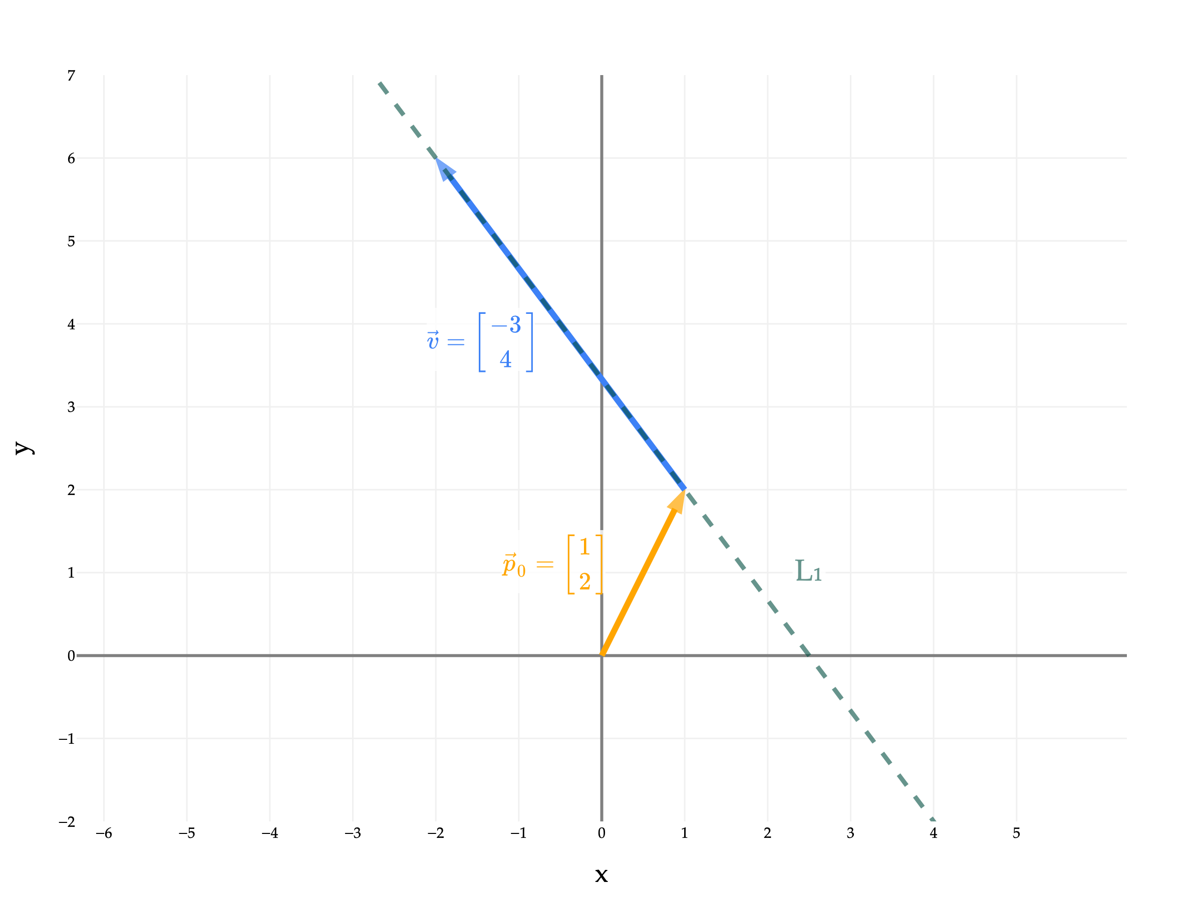
L1=[12]+t[−34],t∈R
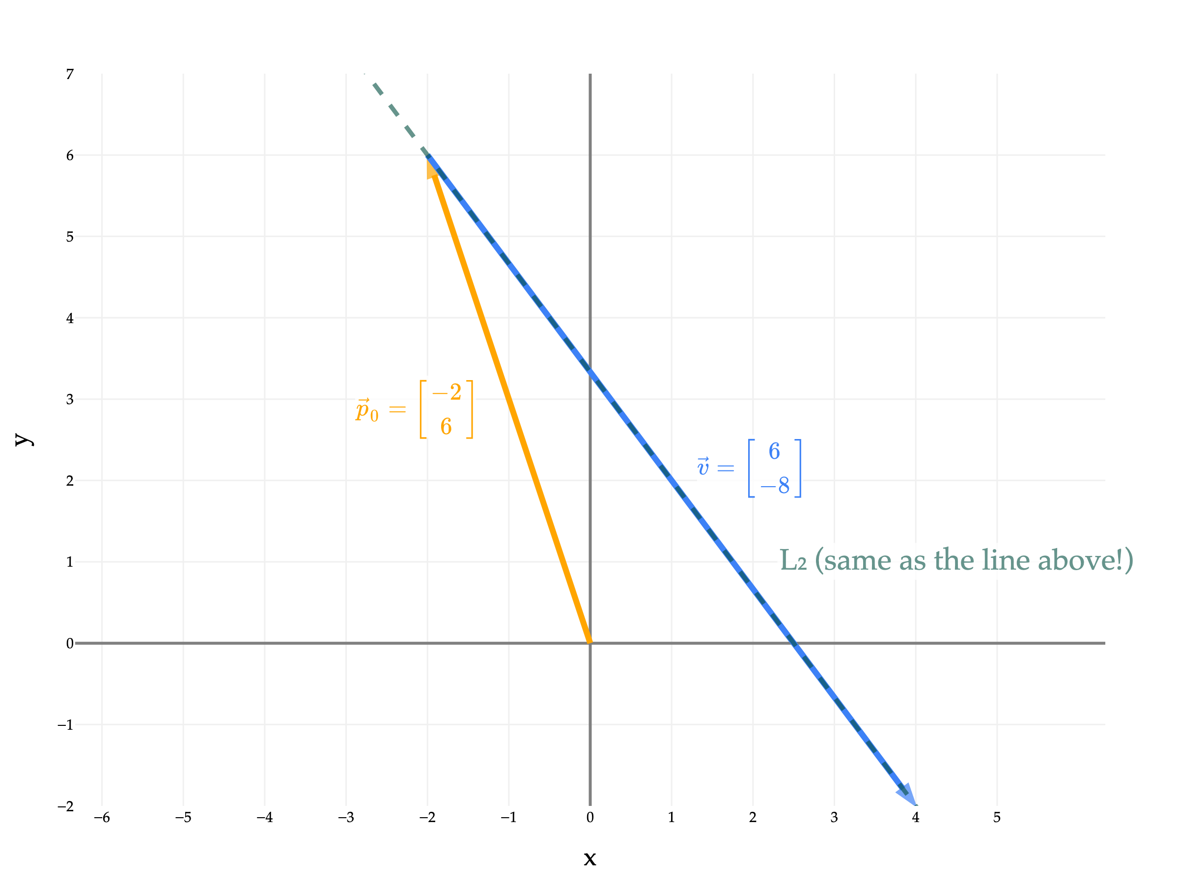
is the same line as
L2=[−26]+t[6−8],t∈R
once you consider all possible values of t in both cases. (I know this is a little confusing, since plugging the same value of t into L1 and into L2 will give you different points, but remember that L1 and L2 are sets, and so we need to consider all possible values of t.)
Below is a plot of L1=[12]+t[−34],t∈R.
from utils import plot_vectors_non_origin

p0 = (1, 2)
v = (-3, 4)

vectors = [
    # ((start_coords, end_coords), color, label)
    (([0, 0], p0), "orange", r"$\vec p_0 = \begin{bmatrix} 1 \\ 2 \end{bmatrix}$"),
    ((p0, tuple(np.array(p0) + np.array(v))), "#3d81f6", r"$\vec v = \begin{bmatrix} -3 \\ 4 \end{bmatrix}$"),
]

fig = plot_vectors_non_origin(vectors, show_axis_labels=True, vdeltax=1.2)

# Focus the plot on x in [-2, 4]
t = np.linspace(-2, 2, 100)  # Solve for t so that x runs from -2 to 4
line_x = p0[0] + t * v[0]
line_y = p0[1] + t * v[1]

fig.add_trace(
    go.Scatter(
        x=line_x,
        y=line_y,
        mode="lines",
        line=dict(color="rgba(0,77,64,0.6)", width=3, dash="dash"),
        showlegend=False,
        hoverinfo="skip",
        zorder=0
    ),
)

# This annotation indicates the line represents all possible linear combinations of v alone
fig.add_annotation(
    x=1.5 * v[0] + 7,
    y=1.5 * v[1] - 5,
    text="L₁",
    showarrow=False,
    font=dict(size=20, color="rgba(0,77,64,0.6)"),
    bgcolor="rgba(255,255,255,0.8)"
)

fig.update_yaxes(
    scaleanchor="x",
    scaleratio=1,
    range=[-2, 7]
)

fig.update_xaxes(
    range=[-4, 4],
    tickvals=np.arange(-6, 6, 1)
)

fig.show(renderer='png', scale=3)
And here’s L2=[−26]+t[6−8],t∈R.
import numpy as np
import plotly.graph_objects as go
from utils import plot_vectors_non_origin

p0 = (-2, 6)
v = (6, -8)

vectors = [
    # ((start_coords, end_coords), color, label)
    (([0, 0], p0), "orange", r"$\vec p_0 = \begin{bmatrix} -2 \\ 6 \end{bmatrix}$"),
    ((p0, tuple(np.array(p0) + np.array(v))), "#3d81f6", r"$\vec v = \begin{bmatrix} 6 \\ -8 \end{bmatrix}$"),
]

fig = plot_vectors_non_origin(vectors, show_axis_labels=True, vdeltax=1.2)

# Focus the plot on x in [-2, 4]
t = np.linspace(-2, 2, 100)  # Solve for t so that x runs from -2 to 4
line_x = p0[0] + t * v[0]
line_y = p0[1] + t * v[1]

fig.add_trace(
    go.Scatter(
        x=line_x,
        y=line_y,
        mode="lines",
        line=dict(color="rgba(0,77,64,0.6)", width=3, dash="dash"),
        showlegend=False,
        hoverinfo="skip",
        zorder=0
    ),
)

# This annotation indicates the line represents all possible linear combinations of v alone
fig.add_annotation(
    x=4.5,
    y=1,
    text="L₂ (same as the line above!)",
    showarrow=False,
    font=dict(size=20, color="rgba(0,77,64,0.6)"),
    bgcolor="rgba(255,255,255,0.8)"
)

fig.update_yaxes(
    scaleanchor="x",
    scaleratio=1,
    range=[-2, 7]
)

fig.update_xaxes(
    range=[-4, 4],
    tickvals=np.arange(-6, 6, 1)
)

fig.show(renderer='png', scale=3)
Note that we end up with the same line, despite the different starting points and direction vectors!
The proceeding activities give you some practice with the parametric form of a line.
Write the line y=−3x+5 in parametric form. There are multiple (infinitely many!) possible answers; give just one.
Solution
The line above passes through the point (0,5) and is parallel to the vector [1−3], since for every 1 unit we move in the x-direction, we move -3 units in the y-direction. So, the line is:
L=[05]+t[1−3],t∈R
To verify that we got the right line, let’s plug in a few values of t and verify that they match the equation y=−3x+5.
When t=0, we get the point (0,5), and −3(0)+5=5 ✅.
When t=1, we get the point (1,2), and −3(1)+5=2 ✅.
When t=−10, we get the point (−10,35), and −3(−10)+5=35 ✅.
(We only need to check two points, since if two lines have the same two points, they must be the same line.)
Could the line you found in Activity 2 be described as the span of a single vector? Why or why not?
Solution
No, because it doesn’t pass through the origin, and the span of a single vector is always a line that passes through the origin.
Let’s look at L once more:
L=⎣⎡5−132⎦⎤+t⎣⎡5−10−2⎦⎤,t∈R
Just by looking at the equation above, we don’t know for a fact that it doesn’t pass through the origin, (0,0,0,0). The fixed point that it is defined relative to, (5,−1,3,2), is not the origin, but the origin might still be on the line if we pick the right value of t.
But, we can verify that that’s not the case by plugging in t=−1, which gives us a 0 in the first two coordinates, but non-zero values in the other coordinates. At t=−1:
L=⎣⎡5−132⎦⎤−1⎣⎡5−10−2⎦⎤=⎣⎡0034⎦⎤
There’s no value of t other than -1 such that 5+t(5)=0, so no other value of t will give us the point (0,0,0,0).
Find the equation of the line, in standard form, that is orthogonal to the line
3x+4y+12=0
and passes through the point (9,5).
Solution
What does it mean for two lines to be orthogonal? In R2 or R3, it’s sufficient to say that they’re orthogonal if they intersect at a right angle, because this is an idea we can visualize.
But more generally, we should think of two lines as orthogonal if their direction vectors are orthogonal when written in parametric form.
That is, L1=p0+tv1 and L2=q0+sv2 are orthogonal if v1⋅v2=0. The values of the starting points don’t change whether the lines are orthogonal, that just changes where they intersect.
Let’s return to our problem, which involves finding a line orthogonal to 3x+4y+12=0. What is this line in parametric form? Rearranging it to slope-intercept form gives us
y=−43x−3
which means that for every 1 unit we move in the x-direction, we move −43 units in the y-direction. So, the direction vector of the line is [1−43], or equivalently, [4−3] (I multiplied by 4 to get nice numbers in the direction vector; as we saw earlier, any non-zero scalar multiple of a direction vector will give us the same line).
You might notice a general pattern from this: the direction vector for the line ax+by+c=0 is [b−a]. I’d avoid memorizing this, though, and would rather you derive it from scratch every time (it’s not a good use of your memory to memorize this).
We want a line orthogonal to 3x+4y+12=0, so we need a direction vector orthogonal to [4−3]. A natural choice is to create a direction vector of [34], since [34]⋅[4−3]=0.
So, in parametric form, one way to express the line we’re looking for is
L=[95]+t[34],t∈R
But we want our new line in standard form, i.e. ax+by+c=0. To get this, we can look at the direction vector of the new line, [34] and recognize that it’s saying to move 4 units in the y-direction for every 3 units we move in the x-direction, implying a slope of 34. The new line we’re looking for then is y=34x+w0, or equivalently 4x−3y+c=0.
To find c, we can plug in the point (9,5) into the equation:
4(9)−3(5)+c=0⟹36−15+c=0⟹c=−21
So, the line we’re looking for is 4x−3y−21=0.
You might also notice that the original line 3x+4y+12=0 has coefficients of 3 and 4 on x and y, and the direction vector of the line orthogonal to it is [34]. Keep this in mind, as it’ll be useful in the section below on planes.
Lines are 1-dimensional objects, whether they exist in R2, or R3, or R47, or in general Rn.
Similarly, planes are 2-dimensional objects. In R2, since there only exist two dimensions in the first place, the entirety of the coordinate system is one single plane, which we call the xy-plane.
Let’s start by building intuition for planes in R3, the most natural setting for them, and then generalize.
Note that both planes are flat surfaces that extend infinitely in all directions. The fact that the blue plane is cut off at the edges is just due to how I’m plotting the planes, not that there’s some boundary within which the plane is defined.
You’ll notice that the blue plane is relatively shallow, while the orange plane is relatively steep. Why?
I find the form z=Ax+By+C easier to understand intuitively, since it shows the rate of change of z with respect to x and y more clearly. Starting with z=Ax+By+C, we have that
∂x∂z=A,∂y∂z=B
In this example, the blue plane has A=53 and B=54, while the orange plane has A=−5 and B=−3, which explains their relative steepness.
That said, be careful, since a plane need not have a non-zero coefficient on z. For example, 3x+4y=0 and 3x+4y=5 is are perfectly valid planes, and they happen to be parallel.
draw_equations([[3, 4, 0, 0], [3, 4, 0, 5]])
Loading...
A key property of planes is that they are flat. Sure, we know that intuitively, but what does it actually mean?
This property is not true in general for other surfaces.
I first mentioned planes back in Chapter 3.1, when we intuitively discussed the fact that the set of all linear combinations of two non-collinear vectors in R3 forms a plane. We discussed this idea at length in Chapter 4.1, too.
So, given two vectors u=⎣⎡u1u2u3⎦⎤,v=⎣⎡v1v2v3⎦⎤∈R3, how do we find the equation of the plane they span, in standard form?
We know that the plane spanned by two vectors in R3 must contain the zero vector, since 0u+0v=0. This means that the point (x,y,z)=(0,0,0) must satisfy the equation of the plane. Plugging in (x,y,z)=(0,0,0) into ax+by+cz+d=0 gives us d=0.
So, I’m searching for a plane of the form ax+by+cz=0. Plugging in u=⎣⎡u1u2u3⎦⎤ tells me that a, b, and c must satisfy
au1+bu2+cu3=0
Similarly, a, b, and c must also satisfy
av1+bv2+cv3=0
Look closely. The left-hand side of both equations looks a lot like the dot product of ⎣⎡abc⎦⎤ with each of u and v. Since those dot products must both be 0 (coming from the right-hand side of each equation), we’re really just looking for a vector ⎣⎡abc⎦⎤ that’s orthogonal to both u and v.
There are infinitely many vectors orthogonal to a particular pair of vectors u and v, meaning there are infinitely many possible values of a, b, and c that satisfy the above equations. (There are 2 equations but 3 unknowns, so we’d expect there to be infinitely many solutions.)
But, one property that all of these vectors share is that they all point in the same direction – if ⎣⎡abc⎦⎤ is orthogonal to u and v, then so is any non-zero scalar multiple of ⎣⎡abc⎦⎤.
from utils import plot_vectors
import numpy as np
import plotly.graph_objects as go

v1 = (5, 2, 1)
v2 = (-2, 3, 0)

fig = plot_vectors([(v1, "orange", r"u"),
                    (v2, "#3d81f6", r"v"),
                    ], show_axis_labels=True, vdeltax=1, vdeltay=1)

# Add the plane spanned by v1 and v2
plane_extent = 20
num_points = 3

s_range = np.linspace(-plane_extent, plane_extent, num_points)
t_range = np.linspace(-plane_extent, plane_extent, num_points)
s_grid, t_grid = np.meshgrid(s_range, t_range)

plane_x = s_grid * v1[0] + t_grid * v2[0]
plane_y = s_grid * v1[1] + t_grid * v2[1]
plane_z = s_grid * v1[2] + t_grid * v2[2]

fig.add_trace(go.Surface(
    x=plane_x,
    y=plane_y,
    z=plane_z,
    opacity=0.8,
    colorscale=[[0, 'rgba(61,129,246,0.3)'], [1, 'rgba(61,129,246,0.3)']],
    showscale=False,
))

# Compute the cross product of v1 and v2
v1_arr = np.array(v1)
v2_arr = np.array(v2)
cross = np.cross(v1_arr, v2_arr)

# Draw the line spanned by the cross product through the origin as a dotted line
line_extent = 10
line_points = np.linspace(-line_extent, line_extent, 2)
line_x = line_points * cross[0]
line_y = line_points * cross[1]
line_z = line_points * cross[2]

fig.add_trace(
    go.Scatter3d(
        x=line_x,
        y=line_y,
        z=line_z,
        mode="lines",
        line=dict(color="rgba(0,77,64,0.6)", width=3, dash="dot"),
        showlegend=False,
        hoverinfo="skip"
    ),
)
# Add annotation at the midpoint of the line in the same color
mid_idx = len(line_points) // 2
fig.add_trace(
    go.Scatter3d(
        x=[5],y=[5],z=[5],
        mode="text",
        text=["All vectors orthogonal to u and v lie on this line"],
        textposition="top center",
        textfont=dict(color="rgba(0,77,64,0.9)", size=14),
        showlegend=False,
        hoverinfo="skip"
    )
)

fig.update_xaxes(
    scaleanchor="y",
    scaleratio=1,
    tickvals=np.arange(-10, 10, 1)
)

fig.update_yaxes(
    scaleanchor="x",
    scaleratio=1,
    tickvals=np.arange(-10, 10, 1)
)

fig.update_layout(
    scene=dict(
        xaxis=dict(range=[-10, 10]),
        yaxis=dict(range=[-10, 10]),
        zaxis=dict(range=[-10, 10]),
        aspectmode='cube',
    ),
    width=600,
    height=600,
    scene_camera=dict(
        eye=dict(x=-1.2, y=2, z=1.2)
    ),
)

fig.show()
Loading...
One particular vector (i.e. set of coefficients a, b, and c) that satisfies the above equations is the cross product of u and v.
There’s a lot of meaning baked into the definition of the cross product, but most of it is more relevant in a traditional engineering or physics context. For example, the cross product is anticommutative, meaning that the order you compute it in matters.
u×v=−(v×u)
That’s the type of statement we won’t bother investigating further here. The key fact that is relevant for us right now is that the vector u×v is orthogonal to both u and v.
The equation of the plane spanned by u and v is then given by
−3x−2y+19z=0
The vector that the cross product returns is sometimes called the normal vector of the plane. Normal is another term for orthogonal or perpendicular. For the plane −3x−2y+19z=0, the normal vector is ⎣⎡−3−219⎦⎤, as that vector is orthogonal to the two vectors u and v that span the plane. When we’re looking at the standard form of the equation of a plane in R3, the normal vector is just the coefficients of x, y, and z in the equation ax+by+cz=0.
There are infinitely many normal vectors for a given plane, since we can multiply any normal vector by a scalar and still get a normal vector. For example, ⎣⎡−3−219⎦⎤ is a normal vector for the plane −3x−2y+19z=0, and so is ⎣⎡−6−438⎦⎤ and ⎣⎡12/3−19/3⎦⎤. Equivalently, −6x−4y+38z=0 and x+32y−319z=0 are ways to write the same plane we’ve been looking at.
The cross product is a construct that only exists in 3-dimensions. Why is that? The cross product relies on the fact that the vectors u and v are linearly independent, meaning they span a plane, and that there is only one direction in R3 that is orthogonal to that plane. The cross product returns a vector in that direction. But, given two vectors in R4, for instance, there are infinitely many directions that are orthogonal to both of those two vectors, so it’s hard to think of an operation that returns any one of them.
All of that is to say, in R4 and above, we can’t express planes in standard form, the same way we can’t express lines in R3 in standard form. Instead, we’ll need to resort to their parametric form.
Again, the formal way of stating this definition is to treat the plane like a set of points that obeys an inclusion condition.
P={p0+su+tv∣s,t∈R}
This definition is very similar to the definition of the parametric form of a line in Rn, it’s just that instead of one direction vector, we have two. For instance,
P=⎣⎡3812−7π⎦⎤+s⎣⎡102−100⎦⎤+t⎣⎡52−1310⎦⎤
is a plane in R6, and you should think of it as a 2-dimensional “slice” of 6-dimensional space.
Prove that if you pick any two points on a plane in Rn, the line connecting the two points is contained entirely on the plane.
Hint: Start by picking two points on the plane. Both of them must satisfy the parametric equation above, just with different values of s and t. Then, using what you’ve learned about parametric equations of lines, find the equation of the line connecting the two. What do you notice about that line?
Consider the points (3,4,5), (1,9,−2), and (2,2,0). Find the equation of the plane that passes through all three points, and express that plane in both parametric form and standard form, ax+by+cz+d=0.
Solution
Start by picking one of the three points; we’ll use (3,4,5). Then, subtract this point from the other two points to find two direction vectors on the plane:
u=⎣⎡19−2⎦⎤−⎣⎡345⎦⎤=⎣⎡−25−7⎦⎤
v=⎣⎡220⎦⎤−⎣⎡345⎦⎤=⎣⎡−1−2−5⎦⎤
So, the plane in parametric form is
P=⎣⎡345⎦⎤+s⎣⎡−25−7⎦⎤+t⎣⎡−1−2−5⎦⎤,s,t∈R
To find the standard form, compute the cross product of the two direction vectors:
So far, we’ve learned how to think of lines and planes in arbitrarily high dimensions. We can’t visualize a plane in R76, but we have some intuition that it’s a 2-dimensional “slice” of 76-dimensional space.
On the topic of slices:
A line is a 1-dimensional “slice” of 2-dimensional space.
A plane is a 2-dimensional “slice” of 3-dimensional space.
In general, a hyperplane is an (n−1)-dimensional “slice” of n-dimensional space.
The most common way of representing a hyperplane is the form a⋅x+b=0.
Example: 2x1+3x2−5=0 is a hyperplane in R2, defined by the vector a=[23] and b=−5. This is just a line in R2. (If it helps to see that this is a line, relabel x1 and x2 as x and y.)
Example: x1+x2+x3=0 is a hyperplane in R3, defined by the vector a=⎣⎡111⎦⎤ and b=0. This is just a plane in R3.
Hyperplanes are hugely important in machine learning, particularly in the context of classification. You should think of a hyperplane in Rn as a boundary that divides all of Rn into two halves: everything is either above it or below it.
For example, the hyperplane ⎣⎡−3−219⎦⎤⋅x=0 is shown below. Any point in R3 is either above it, meaning ⎣⎡−3−219⎦⎤⋅x>0, or below it, meaning ⎣⎡−3−219⎦⎤⋅x<0. (Yes, this hyperplane is just the plane −3x−2y+19z=0 from earlier!)
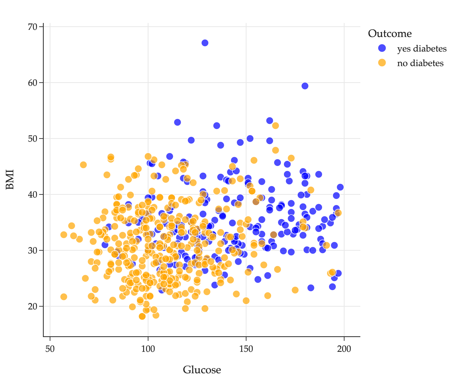
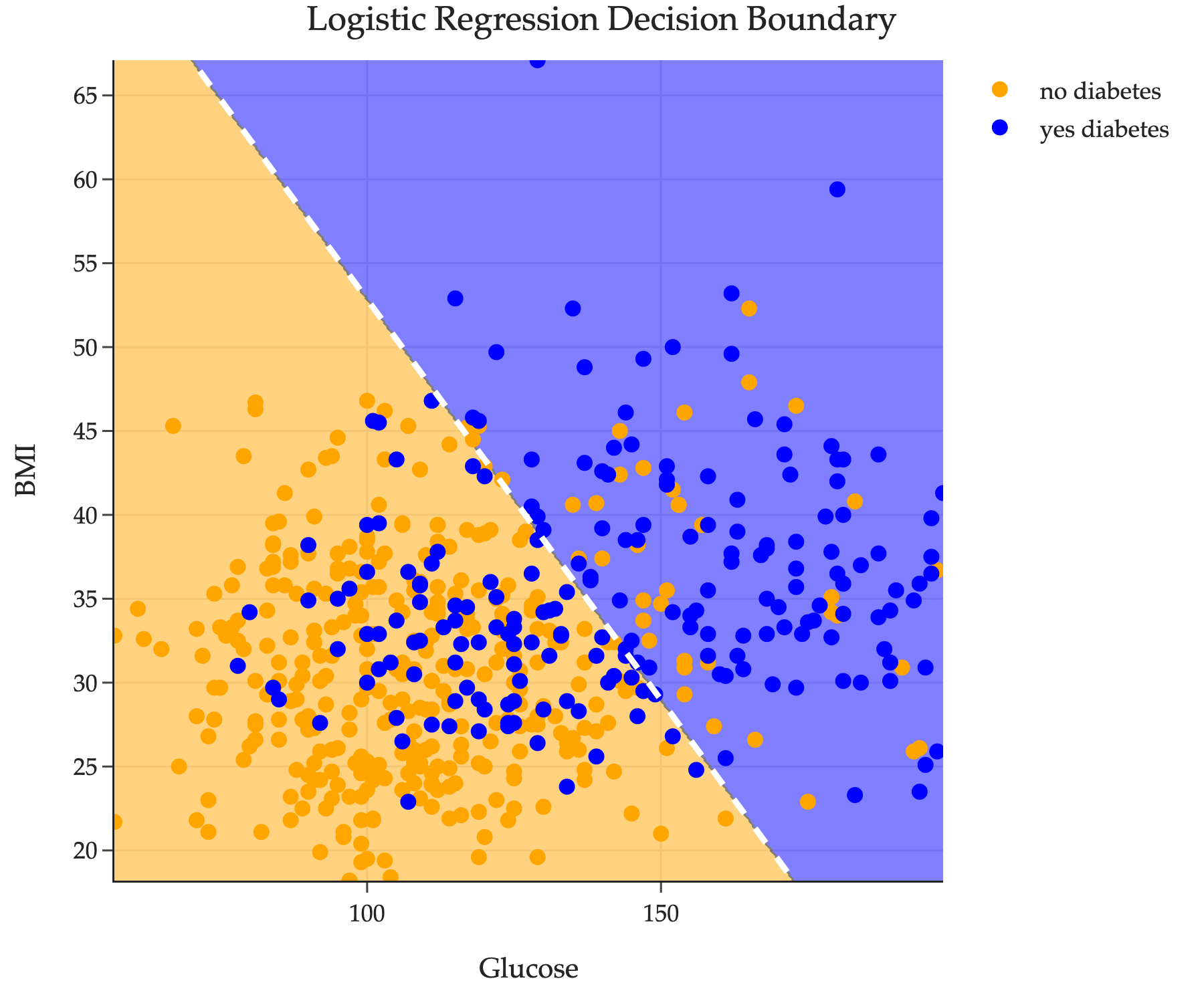
Another more concrete example of a hyperplane comes from looking at the diabetes classification problem first introduced in Homework 3. There, we explored a dataset of several patients, each of which had two features – a glucose level and a body mass index (BMI) – along with a binary label indicating whether they have diabetes or not.
import os
import sys

import pandas as pd
from sklearn.model_selection import train_test_split
from sklearn.linear_model import LogisticRegression

ASSET_DIR = os.path.join('hyperplane-ex')
if ASSET_DIR not in sys.path:
    sys.path.append(ASSET_DIR)
import util

diabetes = pd.read_csv(os.path.join(ASSET_DIR, 'data', 'diabetes.csv'))
X_train, X_test, y_train, y_test = train_test_split(
    diabetes[['Glucose', 'BMI']], diabetes['Outcome'], random_state=1
)

fig = util.create_base_scatter(X_train, y_train)
fig.update_layout(
    title='',
    font=dict(family='Palatino'),
    width=600
)
fig.show(renderer='png', scale=3)
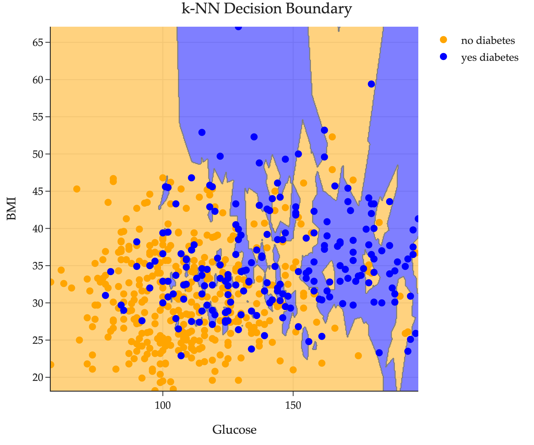
In a homework assignment, we introduce the k-nearest neighbors (k-NN) classifier. You might recall that the decision boundary of a k-NN classifier looks like a bunch of irregularly shaped blobs in the feature space (R2 here).
Another common family of classifiers is linear classifiers, where the decision boundary is a hyperplane. One such linear classifier is the logistic regression classifier. On this dataset, its decision boundary is plotted below.
import warnings
warnings.filterwarnings('ignore')
model = LogisticRegression()
model.fit(X_train, y_train)

fig = util.show_decision_boundary(model, X_train, y_train, title='', grid_n=500)
fig.update_layout(
    title='Logistic Regression Decision Boundary',
    font=dict(family='Palatino'),
    width=600
)

# Draw a dotted white line on the decision boundary
import numpy as np

# Get the coefficients for the decision boundary: w1 * x1 + w2 * x2 + b = 0
coef = model.coef_[0]
intercept = model.intercept_[0]

import plotly.graph_objects as go
# x1 will range from min to max Glucose value in the training set
x1_vals = np.linspace(X_train['Glucose'].min(), X_train['Glucose'].max(), 200)
# x2 = (-b - w1*x1)/w2
x2_vals = (-intercept - coef[0] * x1_vals) / coef[1]

fig.add_trace(
    go.Scatter(
        x=x1_vals,
        y=x2_vals,
        mode='lines',
        line=dict(color='white', dash='dash', width=3),
        name='',
    ),
)

fig.show(renderer='png', scale=3)
Here the decision boundary looks like a line because the data is only 2-dimensional, but in general (with more than two features) a linear classifier’s decision boundary is a hyperplane in Rn. The w in the decision boundary equation w⋅x+b=0 comes from minimizing empirical risk, for some model and loss function!
We can even peek at the decision boundary:
model = LogisticRegression()
model.fit(X_train, y_train)
Loading...
model.coef_
array([[0.04, 0.08]])
model.intercept_
array([-7.85])
This is telling us that the decision boundary is of the form
0.04⋅Glucosei+0.08⋅BMIi−7.85=0
or
w∗[0.040.08]⋅xi[GlucoseiBMIi]−7.85=0
If this classifier used more features, then the decision boundary would involve more terms. Either way, it would be a hyperplane in Rd, where d is the number of features used. Here, d=2, so the decision boundary is a (d−1)-dimensional hyperplane in R2, i.e. a line in R2.
The specifics of logistic regression and how it works are beyond the scope of our course, and certainly not relevant to this section of the notes. I’ve provided this example here just to give you context for where hyperplanes come up in machine learning.