Drag the plot above to look at all five vectors from different angles. You should notice that all of the linear combinations of $\color{#d81b60}\vec w$ and $\color{#004d40}\vec r$ lie on the same plane! We’ll develop more precise terminology to describe this idea, once again, in Chapter 4.1.

3.2. Norms¶

Earlier in this section, we defined the norm of a vector $\vec v$ as:

\lVert \vec v \rVert = \sqrt{v_1^2 + v_2^2 + \cdots + v_n^2} = \sqrt{\sum_{i=1}^n v_i^2}

Now that we know how to add and scale vectors, we should think about how the norm behaves under these operations.

Properties of the Norm¶

The Three Properties

Recall, for $\vec v \in \mathbb{R}^n$ :

\lVert \vec v \rVert = \sqrt{v_1^2 + v_2^2 + \cdots + v_n^2} = \sqrt{\sum_{i=1}^n v_i^2}

Then, $\lVert \vec v \rVert$ satisfies:

$\lVert \vec v \rVert \geq 0$ , and $\lVert \vec v \rVert = 0$ if and only if $\vec v$ is the zero vector, $\vec 0 = \begin{bmatrix} 0 \\ 0 \\ \vdots \\ 0 \end{bmatrix}$ .
$\lVert c \vec v \rVert = |c| \lVert \vec v \rVert$ for all $c \in \mathbb{R}$ .
$\lVert \vec u + \vec v \rVert \leq \lVert \vec u \rVert + \lVert \vec v \rVert$ .

Properties 1 and 2 are intuitive enough:

Property 1 states that it’s impossible for a vector to have a negative norm. To calculate the norm a vector, we sum the squares of each of the vector’s components. As long as each component $v_i$ is a real number, then $v_i^2 \geq 0$ , and so $\sum_{i=1}^n v_i^2 \geq 0$ . The square root of a non-negative number is always non-negative, so the norm of a vector is always non-negative. The only case in which $\sum_{i=1}^n v_i^2 = 0$ is when each $v_i = 0$ , so the only vector with a norm of 0 is the zero vector.
Property 2 states that scaling a vector by a scalar scales its norm by the absolute value of the scalar. For instance, it’s saying that both $2 \vec v$ and $-2 \vec v$ should be double the length of $\vec v$ . See, at this point, if you can prove why this is the case.

Activity 1

Prove Property 2 of vector norms, i.e. that:

\lVert c \vec v \rVert = |c| \lVert \vec v \rVert

Start by using the definition of the norm of the vector $c \vec v$ .

Once you’ve given it a shot, read the solution below.

Solution

As I suggested, let’s start by expanding the definition of $\lVert c \vec v \rVert$ .

\begin{aligned} \lVert c \vec v \rVert &= \sqrt{(c v_1)^2 + (c v_2)^2 + \cdots + (c v_n)^2} \\ &= \sqrt{c^2 v_1^2 + c^2 v_2^2 + \cdots + c^2 v_n^2} \\ &= \sqrt{c^2 (v_1^2 + v_2^2 + \cdots + v_n^2)} \\ \end{aligned}

At this point, we’d like to remove the $c^2$ from the square root. The issue is that $c^2$ is a non-negative number, but $c$ could either have been positive or negative. So, we need to take the absolute value of $c$ . (Remember, $\sqrt{x^2} = |x|$ , not $\sqrt{x} = x$ .)

Then:

\begin{aligned} \lVert c \vec v \rVert &= \sqrt{c^2 (v_1^2 + v_2^2 + \cdots + v_n^2)} \\ &= |c| \underbrace{\sqrt{v_1^2 + v_2^2 + \cdots + v_n^2}}_{\text{This is just $\lVert \vec v \rVert$!}} \\ &= |c| \lVert \vec v \rVert \end{aligned}

So, we’ve shown that $\lVert c \vec v \rVert = |c| \lVert \vec v \rVert$ . Even though this fact may seem like it “just should be true”, we need to be able to rigorously justify it, and we’ve now done just that.

We now revisit norms in detail, including geometric intuition and alternative norms.

The Triangle Inequality¶

Property 3 is a bit more interesting. As a reminder, it states that:

\lVert \vec u + \vec v \rVert \leq \lVert \vec u \rVert + \lVert \vec v \rVert

This is a famous inequality, generally known as the triangle inequality, and it comes up all the time in proofs. Intuitively, it says that the length of a sum of vectors cannot be greater than the sum of the lengths of the individual vectors – or, more philosophically, a sum cannot be more than its parts. It’s called the triangle inequality because it’s a generalization of the fact that in a triangle, the sum of the lengths of any two sides is greater than the length of the third side.

from utils import plot_vectors_non_origin
import numpy as np

fig = plot_vectors_non_origin([(((0, 0), (3, 1)), 'orange', r'$\vec u$'),
                               (((3, 1), (3 + 4, 1 - 6)), '#3d81f6', r'$\vec v$'),
                               (((0, 0), (7, -5)), 'black', r'$\vec u + \vec v$')
                               ]
                               , vdeltax=0.3, vdeltay=0.9)
fig.update_layout(width=500, height=400, yaxis_scaleanchor="x")
fig.update_xaxes(range=[-1, 6], tickvals=np.arange(-5, 15))
fig.update_yaxes(range=[-8, 4], tickvals=np.arange(-8, 4))
fig.show(config={'displayModeBar': False})

Above:

\lVert {\color{orange}\vec u} \rVert = \sqrt{3^2 + 1^2} = \sqrt{10}

\lVert {\color{#3d81f6}\vec v} \rVert = \sqrt{4^2 + (-6)^2} = \sqrt{52}

\lVert {\color{orange}\vec u} + {\color{#3d81f6}\vec v} \rVert = \sqrt{7^2 + (-5)^2} = \sqrt{74}

And indeed, $\sqrt{74} \approx 8.6$ is less than $\sqrt{10} + \sqrt{52} \approx 10.4$ .

To prove that the triangle inequality holds in general, for any two vectors $\vec u, \vec v \in \mathbb{R}^n$ , we’ll need to wait until Chapter 3.3. We don’t currently have any way to expand the norm $\lVert \vec u + \vec v \rVert$ – but we’ll develop the tools to do so soon. Just keep it in mind for now.

Activity 2

The triangle inequality says that:

\lVert \vec u + \vec v \rVert \leq \lVert \vec u \rVert + \lVert \vec v \rVert

In the example above, we had $\sqrt{74} < \sqrt{10} + \sqrt{52}$ . In other words, there was strict inequality.

Find a pair of vectors $\vec u, \vec v$ (say, in $\mathbb{R}^2$ ) such that the triangle inequality achieves equality, i.e. $\lVert \vec u + \vec v \rVert = \lVert \vec u \rVert + \lVert \vec v \rVert$ .

Unit Vectors and the Norm Ball¶

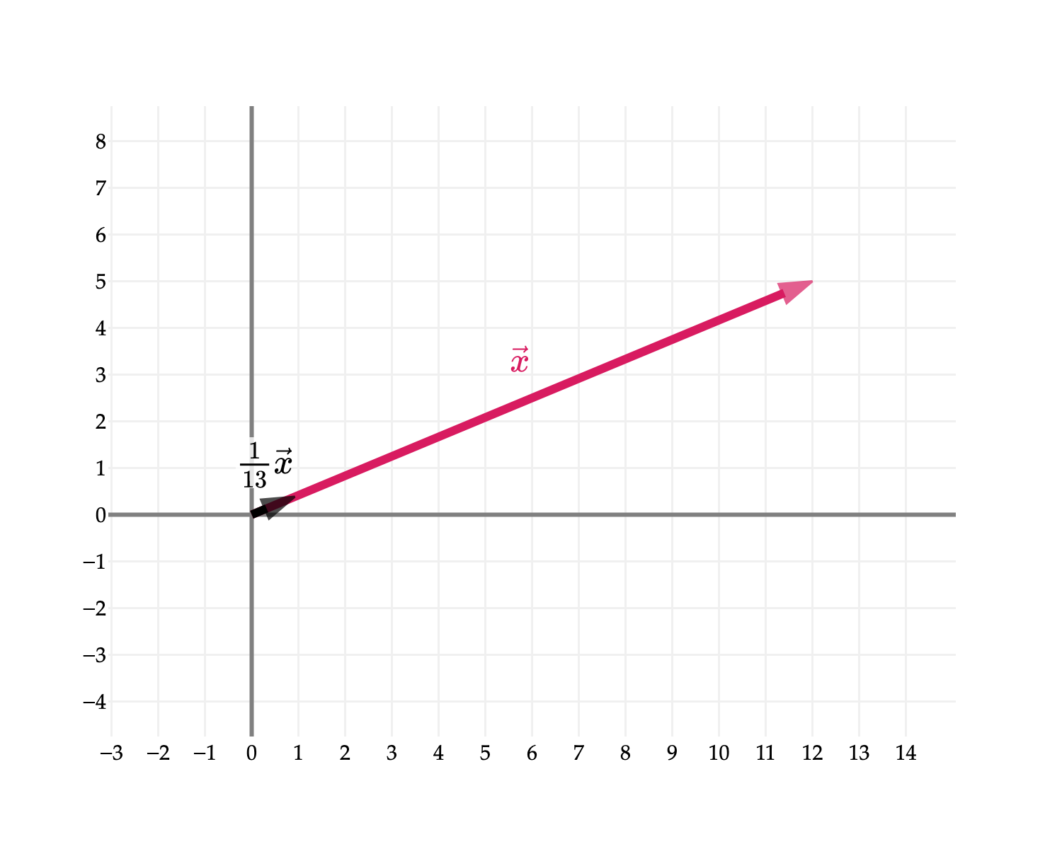
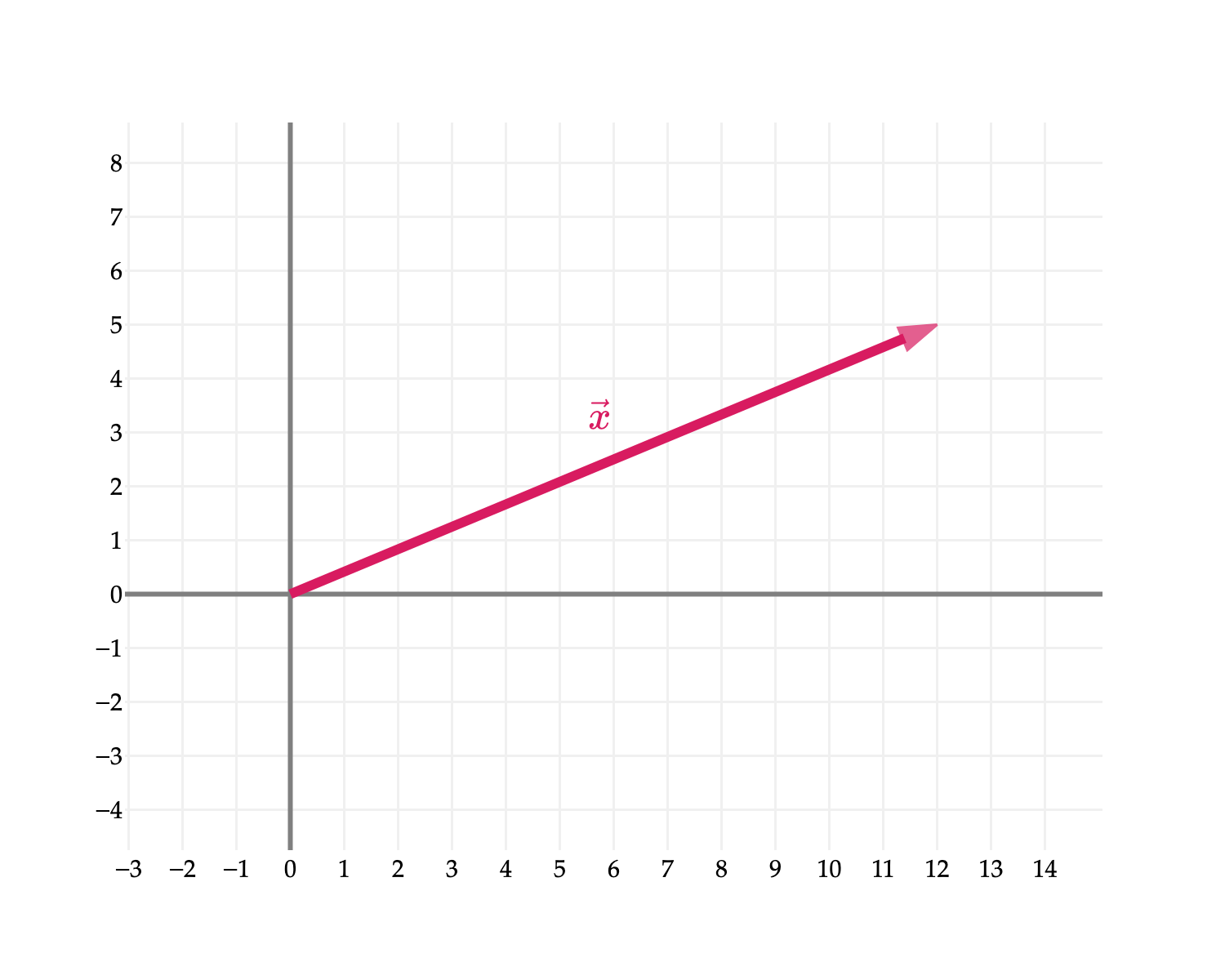
It’s common to use unit vectors to describe directions. I’ll use the same example as in Activity 1, when this idea was first introduced. Consider the vector $\vec x = \begin{bmatrix} 12 \\ 5 \end{bmatrix}$ . Its norm is $\lVert \vec x \rVert = \sqrt{12^2 + 5^2} = \sqrt{169} = \boxed{13}$ . (You might remember the $(5, 12, 13)$ Pythagorean triple from high school algebra– but that’s not important.)

There are plenty of vectors that point in the same direction as $\vec x$ – any vector $c \vec x$ for $c > 0$ does. (If $c < 0$ , then the vector $c \vec x$ points in the opposite direction of $\vec x$ .)

But among all those, the only one with a norm of 1 is $\frac{1}{\boxed{13}} \vec x$ . Property 2 of the norm tells us this.

from utils import plot_vectors
import numpy as np

x = np.array([12, 5])

fig = plot_vectors([(tuple(x), '#d81b60', r'$\vec x$'),
                    (tuple(x / 13), 'black', r'$\frac{1}{13} \vec x$')], vdeltax=0.6, vdeltay=1)
fig.update_layout(width=500, height=400, yaxis_scaleanchor="x")
fig.update_xaxes(range=[-3, 15], tickvals=np.arange(-5, 15))
fig.update_yaxes(range=[-2, 6], tickvals=np.arange(-5, 9))
fig.show(scale=3)

In general, if $\vec v$ is any vector, then:

\frac{\vec v}{\lVert \vec v \rVert}

is a unit vector in the same direction as $\vec v$ . Sometimes, we say that $\frac{\vec v}{\lVert \vec v \rVert}$ is a normalized version of $\vec v$ .

Here’s where things get interesting. Let’s visualize a few vectors and their normalized versions:

\begin{aligned} \vec u &= \begin{bmatrix} 3 \\ 1 \end{bmatrix} \implies \frac{\vec u}{\lVert \vec u \rVert} = \begin{bmatrix} \frac{3}{\sqrt{10}} \\ \frac{1}{\sqrt{10}} \end{bmatrix} \\ \vec v &= \begin{bmatrix} -6 \\ -6 \end{bmatrix} \implies \frac{\vec v}{\lVert \vec v \rVert} = \begin{bmatrix} \frac{-1}{\sqrt{2}} \\ \frac{-1}{\sqrt{2}} \end{bmatrix} \\ \vec w &= \begin{bmatrix} 7 \\ -5 \end{bmatrix} \implies \frac{\vec w}{\lVert \vec w \rVert} = \begin{bmatrix} \frac{7}{\sqrt{74}} \\ \frac{-5}{\sqrt{74}} \end{bmatrix} \\ \vec x &= \begin{bmatrix} -12 \\ 5 \end{bmatrix} \implies \frac{\vec x}{\lVert \vec x \rVert} = \begin{bmatrix} \frac{-12}{13} \\ \frac{5}{13} \end{bmatrix} \\ \vec y &= \begin{bmatrix} -1 \\ -6 \end{bmatrix} \implies \frac{\vec y}{\lVert \vec y \rVert} = \begin{bmatrix} \frac{-1}{\sqrt{37}} \\ \frac{-6}{\sqrt{37}} \end{bmatrix} \\ \end{aligned}

from utils import plot_vectors
import numpy as np

fig = plot_vectors([((3 / np.sqrt(10), 1 / np.sqrt(10)), 'black', r'$\frac{\vec u}{\lVert \vec u \rVert}$'),
                    ((-1 / np.sqrt(2), -1 / np.sqrt(2)), 'black', r'$\frac{\vec v}{\lVert \vec v \rVert}$'),
                    ((7 / np.sqrt(74), -5 / np.sqrt(74)), 'black', r'$\frac{\vec w}{\lVert \vec w \rVert}$'),
                    ((-12 / 13, 5 / 13), 'black', r'$\frac{\vec x}{\lVert \vec x \rVert}$'),
                    ((-1 / np.sqrt(37), -6 / np.sqrt(37)), 'black', r'$\frac{\vec y}{\lVert \vec y \rVert}$')
                    ], vdeltax=0, vdeltay=0)
fig.update_layout(width=400, height=400, yaxis_scaleanchor="x")
fig.update_xaxes(range=[-1.5, 1.5], tickvals=np.arange(-1.5, 1.5, 0.25))
fig.update_yaxes(range=[-1.5, 1.5], tickvals=np.arange(-1.5, 1.5, 0.25))
fig.show(scale=3)

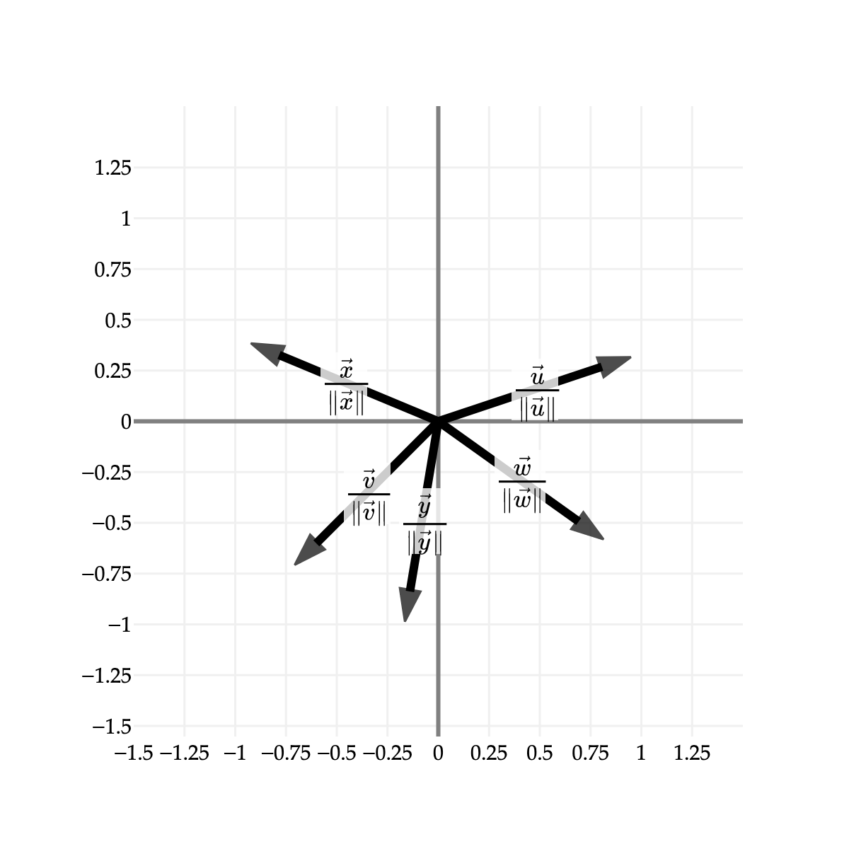
What do these vectors all have in common, other than being unit vectors? They all lie on a circle of radius 1, centered at $(0, 0)$ !

from utils import plot_vectors
import numpy as np
import plotly.graph_objects as go

# Draw the shaded unit circle
theta = np.linspace(0, 2 * np.pi, 200)
x_circle = np.cos(theta)
y_circle = np.sin(theta)

# Add the vectors on top
fig = plot_vectors([((3 / np.sqrt(10), 1 / np.sqrt(10)), 'black', r'$\frac{\vec u}{\lVert \vec u \rVert}$'),
                    ((-1 / np.sqrt(2), -1 / np.sqrt(2)), 'black', r'$\frac{\vec v}{\lVert \vec v \rVert}$'),
                    ((7 / np.sqrt(74), -5 / np.sqrt(74)), 'black', r'$\frac{\vec w}{\lVert \vec w \rVert}$'),
                    ((-12 / 13, 5 / 13), 'black', r'$\frac{\vec x}{\lVert \vec x \rVert}$'),
                    ((-1 / np.sqrt(37), -6 / np.sqrt(37)), 'black', r'$\frac{\vec y}{\lVert \vec y \rVert}$')
                    ], vdeltax=0, vdeltay=0)

# Add dotted circle outline
fig.add_trace(go.Scatter(
    x=x_circle,
    y=y_circle,
    mode="lines",
    line=dict(color="gray", dash="dash", width=3),
    hoverinfo='skip',
    showlegend=False
))

fig.update_layout(width=400, height=400, yaxis_scaleanchor="x")
fig.update_xaxes(range=[-1.5, 1.5], tickvals=np.arange(-1.5, 1.5, 0.5))
fig.update_yaxes(range=[-1.5, 1.5], tickvals=np.arange(-1.5, 1.5, 0.5))
fig.show(scale=3)

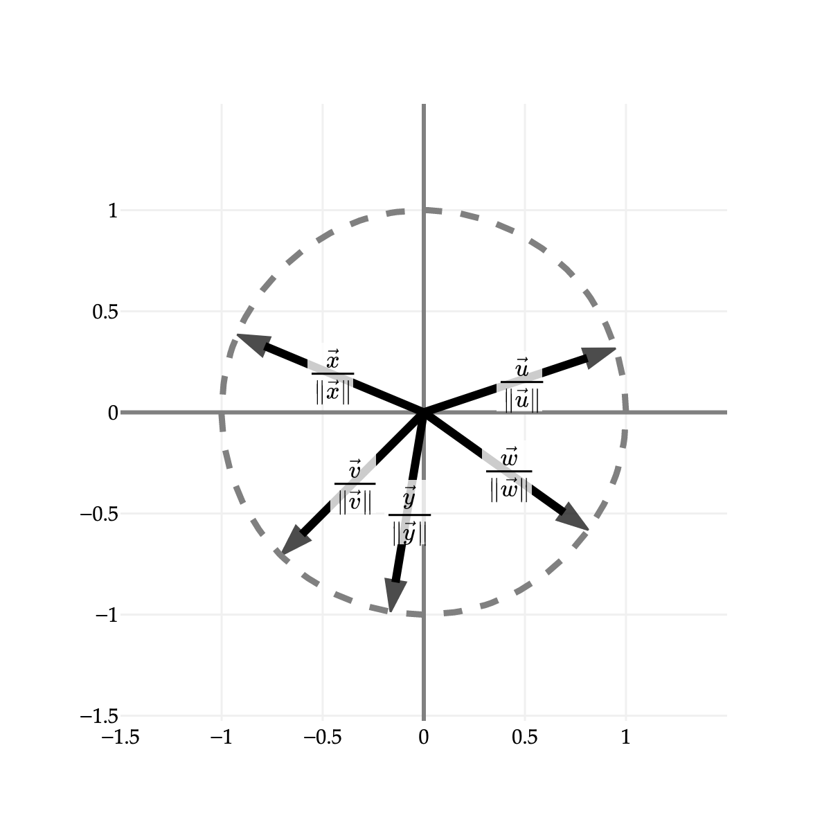
The circle shown above is called the norm ball of radius 1 in $\mathbb{R}^2$ . It shows the set of all vectors $\vec v \in \mathbb{R}^2$ such that $\lVert \vec v \rVert = 1$ . Using set notation, we might say:

\{\vec v : \lVert \vec v \rVert = 1, \vec v \in \mathbb{R}^2\}

That this looks like a circle is no coincidence. The condition $\lVert \vec v \rVert = 1$ is equivalent to $\sqrt{v_1^2 + v_2^2} = 1$ . Squaring both sides, we get $v_1^2 + v_2^2 = 1$ . This is the equation of a circle with radius 1 centered at the origin.

In $\mathbb{R}^3$ , the norm ball of radius 1 is a sphere, and in general, in $\mathbb{R}^n$ , the norm ball of radius 1 is an $n$ -dimensional sphere.

Activity 3

Find the unit vector that points in the same direction as $\vec z = \begin{bmatrix} 4 \\ 0 \\ -3 \\ -3 \end{bmatrix}$ .

Clearly write out all four of its components.

Other Norms¶

So far, we’ve only discussed one “norm” of a vector, sometimes called the $L_{\color{orange}2}$ norm or Euclidean norm. In general, if $\vec v \in \mathbb{R}^n$ is one vector, $\vec v = \begin{bmatrix} v_1 \\ v_2 \\ \vdots \\ v_n \end{bmatrix}$ , then its norm is:

\lVert \vec v \rVert = \sqrt{v_1^{\color{orange}2} + v_2^{\color{orange}2} + \cdots + v_n^{\color{orange}2}} = \sqrt{\sum_{i=1}^n v_i^{\color{orange}2}}

This is, by far, the most common and most relevant norm, and in many linear algebra classes, it’s the only norm you’ll see. But in machine learning, a few other norms are relevant, too, so I’ll briefly discuss them here.

The $L_1$ or Manhattan norm of $\vec v$ is:
$\lVert \vec v \rVert_1 = |v_1| + |v_2| + \cdots + |v_n| = \sum_{i=1}^n |v_i|$
It’s called the Manhattan norm because it’s the distance you would travel if you walked from the origin to $\vec v$ in a grid of streets, where you can only move horizontally or vertically.
The $L_\infty$ or maximum norm of $\vec v$ is:
$\lVert \vec v \rVert_\infty = \max_{i} |v_i|$
This is largest absolute value of any component of $\vec v$ .
For any $p \geq 1$ , the $L_p$ norm of $\vec v$ is:
$\lVert \vec v \rVert_p = \left( \sum_{i=1}^n |v_i|^p \right)^{\frac{1}{p}}$
Note that when $p = 2$ , this is the same as the $L_2$ norm. For other values of $p$ , this is a generalization. Something to think about: why is there an absolute value in the definition?

All of these norms measure the length of a vector, but in different ways. This might ring a bell: we saw very similar tradeoffs between squared and absolute losses in Chapter 1.

Believe it or not, all three of these norms satisfy the same “Three Properties” we discussed earlier.

Back to $\vec x = \begin{bmatrix} 12 \\ 5 \end{bmatrix}$ . What are the $L_2$ , $L_1$ , and $L_\infty$ norms of $\vec x$ ?

from utils import plot_vectors
import numpy as np

x = np.array([12, 5])

fig = plot_vectors([(tuple(x), '#d81b60', r'$\vec x$')], vdeltax=0.6, vdeltay=1)
fig.update_layout(width=500, height=400, yaxis_scaleanchor="x")
fig.update_xaxes(range=[-3, 15], tickvals=np.arange(-5, 15))
fig.update_yaxes(range=[-2, 6], tickvals=np.arange(-5, 9))
fig.show(scale=3)

Here:

$\lVert \vec x \rVert_2 = \sqrt{12^2 + 5^2} = \sqrt{144 + 25} = \sqrt{169} = 13$
$\lVert \vec x \rVert_1 = |12| + |5| = 12 + 5 = 17$
$\lVert \vec x \rVert_\infty = \max(|12|, |5|) = 12$

Let’s revisit the idea of a norm ball. Using the standard $L_2$ norm, the norm ball in $\mathbb{R}^2$ is a circle. What does the norm ball look like for the $L_1$ and $L_\infty$ norms? Or $L_p$ with an arbitrary $p$ ?

import numpy as np
import plotly.graph_objects as go
from plotly.subplots import make_subplots

theta = np.linspace(0, 2 * np.pi, 400)

# L1 norm ball (diamond)
x_l1 = np.cos(theta) / (np.abs(np.cos(theta)) + np.abs(np.sin(theta)))
y_l1 = np.sin(theta) / (np.abs(np.cos(theta)) + np.abs(np.sin(theta)))

# L1.3 norm ball
p13 = 1.3
x_l13 = np.cos(theta)
y_l13 = np.sin(theta)
norm_l13 = (np.abs(x_l13) ** p13 + np.abs(y_l13) ** p13) ** (1/p13)
x_l13 = x_l13 / norm_l13
y_l13 = y_l13 / norm_l13

# L2 norm ball (unit circle)
x_l2 = np.cos(theta)
y_l2 = np.sin(theta)

# L-infinity norm ball (square)
x_linf = np.empty_like(theta)
y_linf = np.empty_like(theta)
for i, t in enumerate(theta):
    c, s = np.cos(t), np.sin(t)
    if np.abs(c) > np.abs(s):
        x_linf[i] = np.sign(c)
        y_linf[i] = np.tan(t) * np.sign(c)
    else:
        y_linf[i] = np.sign(s)
        x_linf[i] = 1/np.tan(t) * np.sign(s)
    norm_inf = max(abs(x_linf[i]), abs(y_linf[i]))
    x_linf[i] /= norm_inf
    y_linf[i] /= norm_inf

fig = make_subplots(
    rows=2, cols=2,
    subplot_titles=[r"$L_1 \text{ norm ball}$", r"$L_{1.3} \text{ norm ball}$", r"$L_2 \text{ norm ball}$", r"$L_\infty \text{ norm ball}$"],
    horizontal_spacing=0.08, vertical_spacing=0.13
)

line_style = dict(color="#888", dash="dash", width=3)

fig.add_trace(go.Scatter(
    x=x_l1, y=y_l1, mode="lines",
    line=line_style, hoverinfo='skip', showlegend=False
), row=1, col=1)

fig.add_trace(go.Scatter(
    x=x_l13, y=y_l13, mode="lines",
    line=line_style, hoverinfo='skip', showlegend=False
), row=1, col=2)

fig.add_trace(go.Scatter(
    x=x_l2, y=y_l2, mode="lines",
    line=line_style, hoverinfo='skip', showlegend=False
), row=2, col=1)

fig.add_trace(go.Scatter(
    x=x_linf, y=y_linf, mode="lines",
    line=line_style, hoverinfo='skip', showlegend=False
), row=2, col=2)

for r in range(1, 3):
    for c in range(1, 3):
        fig.update_xaxes(
            range=[-1.5, 1.5], tickvals=np.arange(-1.5, 1.6, 0.5),
            row=r, col=c, showgrid=True, zeroline=True, gridcolor="#f0f0f0", zerolinecolor="#808080",
            showticklabels=(False if r * c > 1 else True), title=None
        )
        fig.update_yaxes(
            range=[-1.5, 1.5], tickvals=np.arange(-1.5, 1.6, 0.5),
            row=r, col=c, showgrid=True, zeroline=True, gridcolor="#f0f0f0", zerolinecolor="#808080",
            scaleanchor=f"x{2*(r-1)+c}", showticklabels=(False if r * c > 1 else True), title=None
        )

fig.update_layout(
    width=700, height=600,
    plot_bgcolor="white",
    paper_bgcolor="white",
    font=dict(family="Palatino", size=16, color="#222"),
    margin=dict(l=10, r=10, t=40, b=10),
)

fig.show(scale=3)

The $L_1$ norm ball looks like a diamond. Any vector with an $L_1$ norm of 1 will lie on the boundary of the ball. The $L_\infty$ norm ball looks like a square, and the $L_{1.3}$ norm ball looks like a diamond with rounded corners.

This is not the last you’ll see of these norm balls – in particular, in future machine learning courses, you’ll see them again in the context of regularization, which is a technique for preventing overfitting in our models.

Activity 4

In the case of $\vec x = \begin{bmatrix} 12 \\ 5 \end{bmatrix}$ , the $L_1$ norm ( $12 + 5 = 17$ ) is greater than the $L_2$ norm ( $\sqrt{12^2 + 5^2} = \sqrt{169} = 13$ ), i.e. $\lVert \vec x \rVert_1 > \lVert \vec x \rVert_2$ .

Find a vector $\vec y \in \mathbb{R}^2$ such that $\lVert \vec y \rVert_1 = \lVert \vec y \rVert_2$ .
Try and find a vector $\vec z \in \mathbb{R}^2$ such that $\lVert \vec z \rVert_1 < \lVert \vec z \rVert_2$ . What do you encounter?
Prove that $\lVert \vec x \rVert_2 \leq \sqrt{n} \lVert \vec x \rVert_\infty$ for any vector $\vec x \in \mathbb{R}^n$ . (Hint: Start with the definition of the $L_2$ norm of $\vec x$ , square it, and try and compare each element in the sum to the largest element in the vector.)

`np.linalg.norm` and Vectorization¶

It’s been a while since we’ve experimented with numpy. A few things:

As we’ve seen, arrays can be added element-wise by default.
Arrays can also be multiplied by scalars out-of-the-box, meaning that linear combinations of arrays (vectors) are easy to compute. The above two facts mean that array operations are vectorized: they are applied to each element of the array in parallel, without needing to use a for-loop.
To compute the ( $L_2$ ) norm of an array (vector), we can use np.linalg.norm.

Suppose you didn’t know about np.linalg.norm. There’s another way to compute the norm of an array (vector), that doesn’t involve a for-loop. Follow the activity to discover it.

Activity 5

In the cell above:

Write u ** 2. Squaring a vector is not an operation we’ve discussed (and isn’t an operation that exists in math), but numpy gives you back another array. What does this array contain?
Using np.sum and the new array you just created, find the norm of u without using np.linalg.norm.
Find the norm of 3 * u - 0.5 * v using the same technique, and make sure you get the same result as was already displayed for you.

In general, we’ll want to avoid Python for-loops in our code when there are numpy-native alternatives, as these numpy functions are optimized to use C (the programming language) under the hood for speed and memory efficiency.