Symmetric matrices – that is, square matrices where – behave really nicely through the lens of eigenvectors, and understanding exactly how they work is key to Chapter 10.1, when we generalize beyond square matrices.
While editing these notes, I came across a fitting tweet:
Most people with “AI/ML” in their bios don’t even know a real symmetric matrix always has real eigenvalues.
vixhaℓ (@TheVixhal) March 29, 2026
The Spectral Theorem
If you search for the spectral theorem online, you’ll often just see Statement 4 above; I’ve broken the theorem into smaller substatements to see how they are chained together.
The proof of Statement 1 is beyond our scope, since it involves fluency with complex numbers. If the term “complex conjugate” means something to you, read the proof here – it’s relatively short.
The key idea to prove is Statement 2: that for a symmetric matrix, eigenvectors corresponding to different eigenvalues are orthogonal. Suppose is an eigenvector of with eigenvalue and is an eigenvector of with eigenvalue , where . Then
Consider the dot product . Using the fact that is an eigenvector, we get
But we can also rewrite the same quantity using the fact that is symmetric:
So,
which means
Since , the first factor is non-zero, so we must have . Therefore, eigenvectors corresponding to different eigenvalues are orthogonal.
For a given eigenvector direction, we can pick any vector in that direction to be the eigenvector we store in the that we use to diagonalize – if is an eigenvector, so is , , , and so on. The convenient choice is to pick unit vectors in each direction. If we take these unit eigenvectors and place them in the columns of a matrix, that matrix is an orthogonal matrix! Orthogonal matrices satisfy , meaning their columns (and rows) are orthonormal, not just orthogonal to one another. The fact that means that , so taking the transpose of a matrix is the same as taking its inverse.
we’ve “upgraded” to
This is the main takeaway of the spectral theorem: that symmetric matrices can be diagonalized by an orthogonal matrix. Sometimes, is called the spectral decomposition of , but all it is is a special case of the eigenvalue decomposition for symmetric matrices.
Visualizing the Spectral Theorem
Why do we prefer over ? Taking the transpose of a matrix is much easier than inverting it, so actually working with is easier.
But it’s also an improvement in terms of interpretation: remember that orthogonal matrices are matrices that represent rotations. So, if is symmetric, then the linear transformation is a sequence of rotations and stretches.
Let’s make sense of this visually. Consider the symmetric matrix .
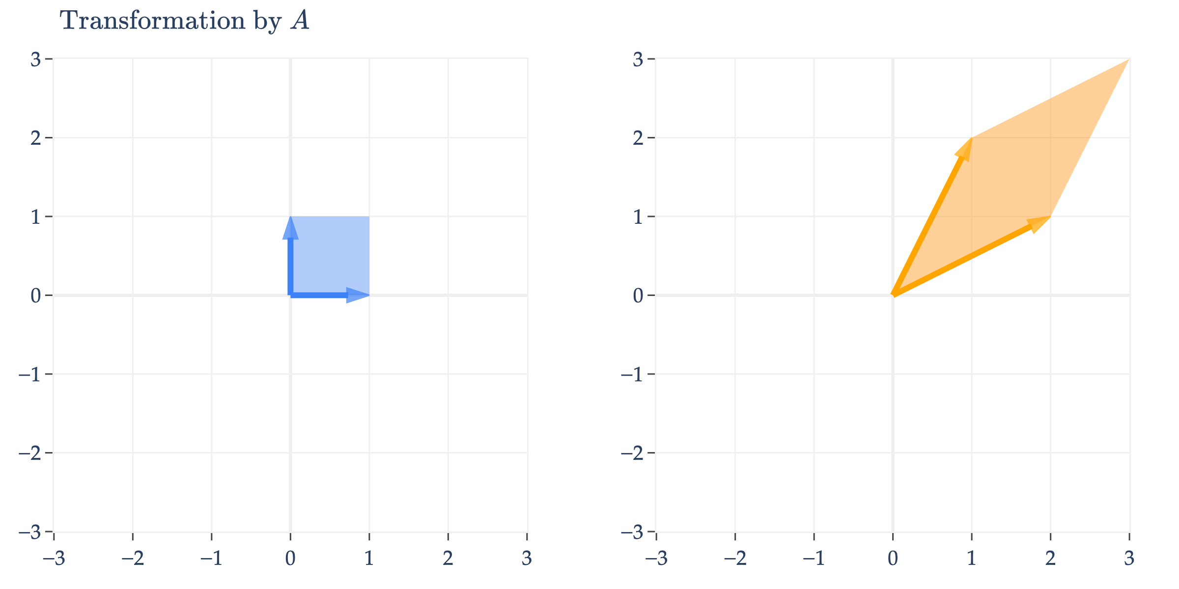
appears to perform an arbitrary transformation; it turns the unit square into a parallelogram, as we first saw in Chapter 6.1.
But, since is symmetric, it can be diagonalized by an orthogonal matrix, .
has eigenvalues with eigenvector and with eigenvector . But, the ’s I’ve written aren’t unit vectors, which they need to be in order for to be orthogonal. So, we normalize them to get and . Placing these ’s as columns of , we get
and so
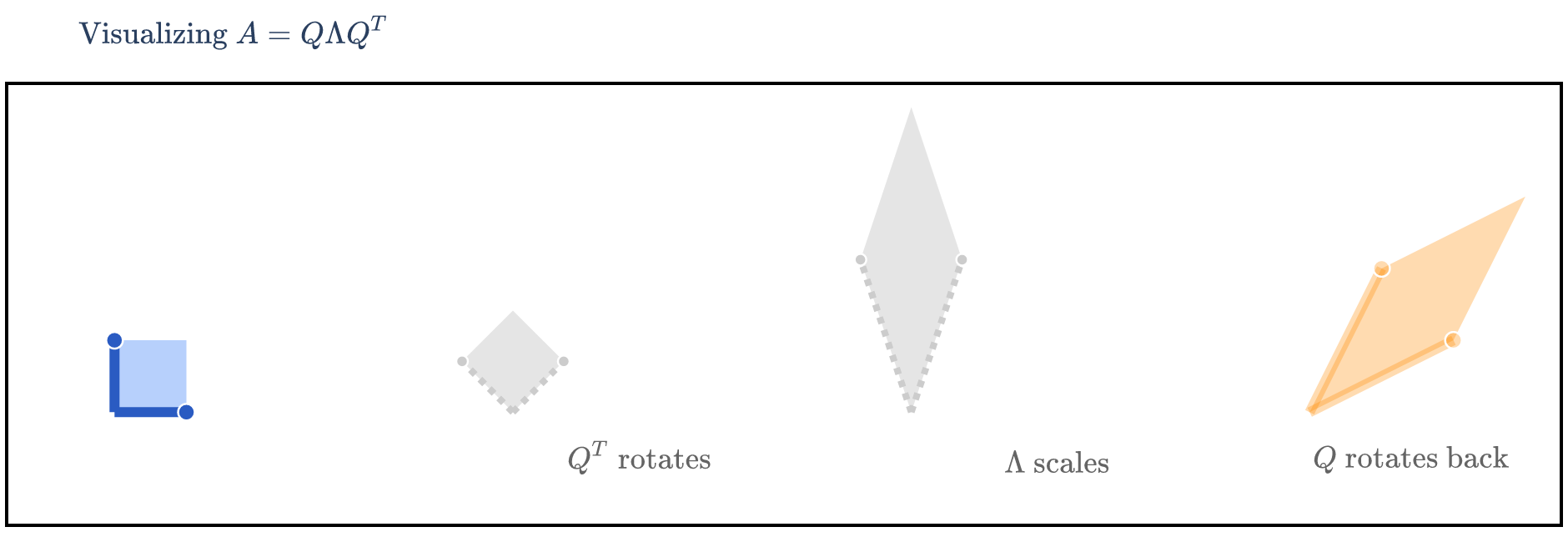
We’re visualizing how turns into , i.e. how turns into . This means that we first need to consider the effect of on , then the effect of on that result, and finally the effect of on that result – that is, read the matrices from right to left.
The Ellipse Perspective
Another way of visualizing the linear transformation of a symmetric matrix is to consider its effect on the unit circle, not the unit square. Below, I’ll apply to the unit circle.
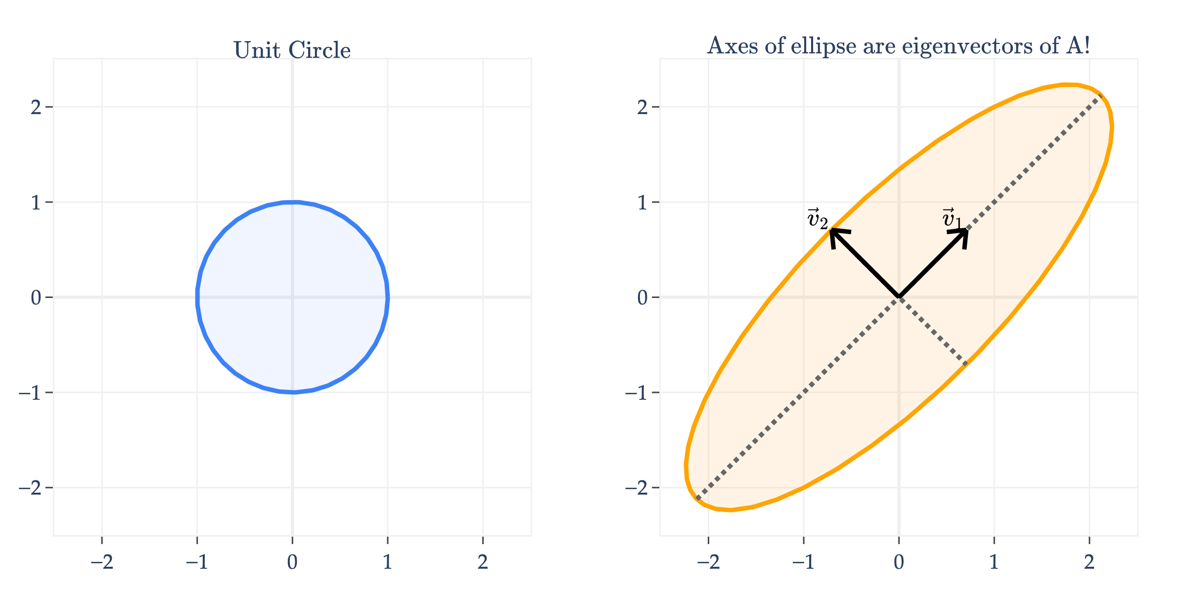
Notice that transformed the unit circle into an ellipse. What’s more, the axes of the ellipse are the eigenvector directions of !
Why is one axis longer than the other? As you might have guessed, the longer axis – the one in the direction of the eigenvector – corresponds to the larger eigenvalue. Remember that has and , so the “up and to the right” axis is three times longer than the “down and to the right” axis, defined by .
Why does this happen? Since is symmetric, it has a spectral decomposition , where is orthogonal and is diagonal. For any vector , let . Then
Now imagine that lies on one of ’s eigenvector directions, say the direction of . In that case, after rotating by , the vector has only one non-zero coordinate, namely the coordinate corresponding to . So the sum above collapses to
Similarly, along the eigenvector direction of , we get . The size of the output along each principal axis is therefore controlled by the corresponding eigenvalue. Larger eigenvalues produce longer axes, and smaller eigenvalues produce shorter axes. Here, and , so the axis in the direction is longer in magnitude than the axis in the direction.
Key Takeaways
The eigenvalue decomposition of a matrix is a decomposition of the form
where is a matrix containing the eigenvectors of as columns, and is a diagonal matrix of eigenvalues in the same order. Only diagonalizable matrices can be decomposed in this way.
The algebraic multiplicity of an eigenvalue is the number of times appears as a root of the characteristic polynomial of .
The geometric multiplicity of is the dimension of the eigenspace of , i.e. .
The matrix is diagonalizable if and only if any of these equivalent conditions are true:
has linearly independent eigenvectors.
For every eigenvalue , . When is diagonalizable, it has an eigenvalue decomposition, .
If is a symmetric matrix, then the spectral theorem tells us that can be diagonalized by an orthogonal matrix such that
and that all of ’s eigenvalues are guaranteed to be real.
What’s next? There’s the question of how any of this relates to real data. Real data comes in rectangular matrices, not square matrices. And even it were square, how does any of this enlighten us?