Eigenvalues and eigenvectors are powerful concepts, but unfortunately, they only apply to square matrices. It would be nice if we could extend some of their utility to non-square matrices, like matrices containing real data, which typically have many more rows than columns.
Introduction
This is precisely where the singular value decomposition (SVD) comes in. You should think of it as a generalization of the eigenvalue decomposition, , to non-square matrices. When we first introduced eigenvalues and eigenvectors, we said that an eigenvector of is a vector whose direction is unchanged when multiplied by – all that happens to is that it’s scaled by a factor of .
But now, suppose is some matrix. For any vector , the vector is in , not , meaning and live in different universes. So, it can’t make sense to say that results from stretching .
Instead, we’ll find pairs of singular vectors, and , such that
where is a singular value of (not a standard deviation!). Intuitively, this says that when is multiplied by , the result is a scaled version of . These singular values and vectors are the focus of this chapter. Applications of the singular value decomposition will start in Chapter 10.2 – but go scroll to the bottom of that section if you want to see what we’re working towards.
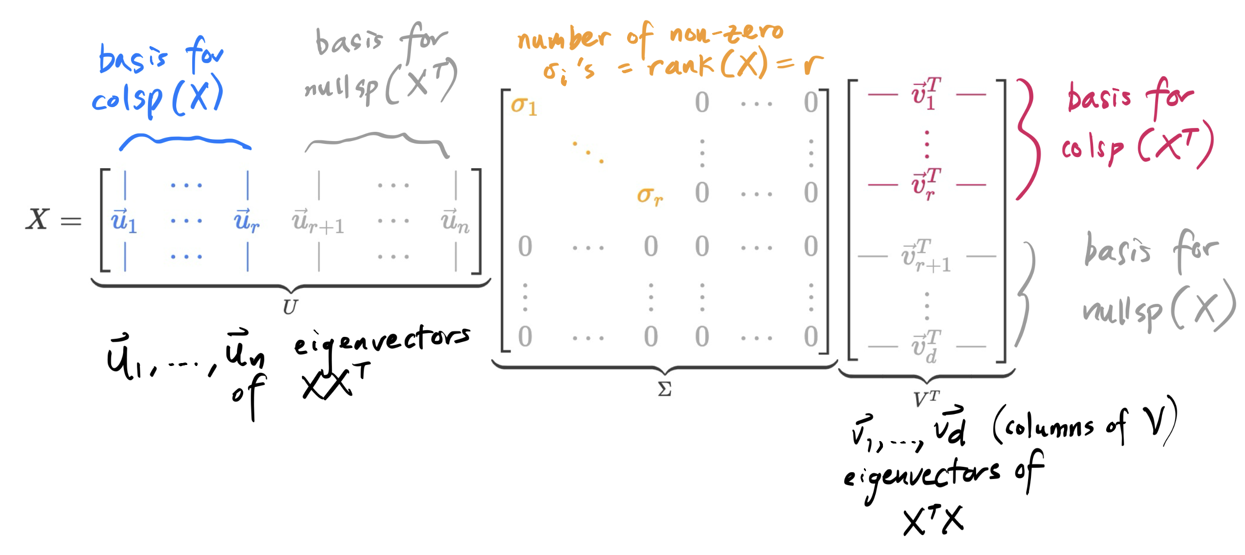
Think of , , and – or perhaps better , , and – as a trio of friends that appear together in the SVD of ; each matrix has such trios, where is the rank of .
I’ll start by giving you the definition of the SVD, and then together we’ll figure out where it came from.
Firstly, note that the SVD exists, no matter what is: it can be non-square, and it doesn’t even need to be full rank. But note that unlike in the eigenvalue decomposition, where we decomposed using just one eigenvector matrix and a diagonal matrix , here we need to use two singular vector matrices and and a diagonal matrix .
There’s a lot of notation and new concepts above. Let’s start with an example, then try and understand where each piece in comes from and means. Suppose
is a matrix with , since its third column is the sum of the first two. Its singular value decomposition is given by :
Two important observations:
and are both orthogonal matrices, meaning and .
contains the singular values of on the diagonal, arranged in decreasing order. We have that , , and . has three singular values, but only two are non-zero. In general, the number of non-zero singular values is equal to the rank of .
Where did all of these numbers come from?
Discovering the SVD
The SVD of depends heavily on the matrices and . While itself is ,
is a symmetric matrix, containing the dot products of ’s columns
is a symmetric matrix, containing the dot products of ’s rows
Since and are both square matrices, they have eigenvalues and eigenvectors. And since they’re both symmetric, their eigenvectors for different eigenvalues are orthogonal to each other, as the spectral theorem guarantees for any symmetric matrix .
Singular Values and Singular Vectors
The singular value decomposition involves creatively using the eigenvalues and eigenvectors of and . Suppose is the SVD of . Then, using the facts that and , we have:
This just looks like we diagonalized and ! The expressions above are saying that:
’s columns are the eigenvectors of
’s columns are the eigenvectors of
and usually have different sets of eigenvectors, which is why and are generally not the same matrix (they don’t even have the same shape).
The eigenvalues of and are the same, though: those are the non-zero entries of and . Since is an matrix, is a matrix and is an matrix. But, when you work out both products, you’ll notice that their non-zero values are the same.
Suppose for example that . Then,
But, these matrices with the squared terms are precisely the 's in the spectral decompositions of and . This means that
where is a singular value of and is an eigenvalue of or .
The above derivation is enough to justify that the eigenvalues of and are never negative, but for another perspective, note that both and are positive semidefinite, meaning their eigenvalues are non-negative. (You’re wrestling with this fact in Lab 11 and Homework 10.)
Another proof that and have the same non-zero eigenvalues
Above, we implicitly used the fact that and have the same non-zero eigenvalues. Here’s a proof of this fact that has nothing to do with the SVD.
Suppose is an eigenvector of with eigenvalue .
What happens if we multiply both sides on the left by ?
Creatively adding parentheses gives us
This shows that is an eigenvector of with eigenvalue . The important thing is that the eigenvalue is shared. This logic can be reversed too, to show that if is an eigenvector of with eigenvalue , then is also an eigenvalue of .
Computing the SVD
To find , , and , we don’t actually need to compute both and : all of these quantities can be uncovered just with one of them.
Let’s return to our example, . Using what we’ve just learned, let’s find , , and ourselves. has fewer entries than , so let’s start with it. I will delegate some number crunching to numpy.
import numpy as np
X = np.array([[3, 2, 5],
[2, 3, 5],
[2, -2, 0],
[5, 5, 10]])
X.T @ Xarray([[ 42, 33, 75],
[ 33, 42, 75],
[ 75, 75, 150]])is a matrix, but its rank is 2, meaning it will have an eigenvalue of 0. What are its other eigenvalues?
eigvals, eigvecs = np.linalg.eig(X.T @ X)
eigvalsarray([225., 9., 0.])The eigenvalues of are 225, 9, and 0. This tells us that the singular values of are , , and 0. So far, we’ve discovered that . Remember that always has the same shape as (both are ), and all of its entries are 0 except for the singular values, which are arranged in decreasing order on the diagonal, starting with the largest singular value in the top left corner.
Let’s now find the eigenvectors of – that is, the right singular vectors of – which we should store in . We expect the eigenvectors of to be orthogonal, since is symmetric.
X.T @ Xarray([[ 42, 33, 75],
[ 33, 42, 75],
[ 75, 75, 150]])For , one eigenvector is , since
For , one eigenvector is , since
For , one eigenvector is , since
Note that is a basis for , since and . Hold that thought for now.
To create , all we need to do is turn , , and into unit vectors.
Stacking these unit vectors together gives us :
And indeed, since is symmetric, is orthogonal: .
Great! We’re almost done computing the SVD. So far, we have
and 
Ideally, we can avoid having to compute the eigenvectors of to stack into . And we can. If we start with
and multiply both sides on the right by , we uncover a relationship between the columns of and the columns of .
Let’s unpack this. On the left, the matrix is made up of multiplying by each column of .
On the right, is made up of stretching each column of by the corresponding singular value in the diagonal of .
But, since , we have
Crucially though, only holds when we’ve arranged the singular values and vectors in , , and consistently. This is one reason why we always arrange the singular values in in decreasing order.
Back to our example. Again, we currently have
We know , and we know each and . Rearranging gives us
which is a recipe for computing , , and .
Something is not quite right: , which means we can’t use to compute . And, even if we could, this recipe tells us nothing about , which we also need to find, since is .
Null Spaces Return
So far, we’ve found two of the four columns of .
The issue is that we don’t have a recipe for what and should be. This problem stems from the fact that .
If we were to compute , whose eigenvectors are the columns of , we would have seen that it has an eigenvalue of 0 with geometric (and algebraic) multiplicity 2.
X @ X.Tarray([[ 38, 37, 2, 75],
[ 37, 38, -2, 75],
[ 2, -2, 8, 0],
[ 75, 75, 0, 150]])eigvals, eigvecs = np.linalg.eig(X @ X.T)
eigvals
array([225., 9., -0., 0.])So, all we need to do is fill and with two orthonormal vectors that span the eigenspace of for eigenvalue 0. is already an eigenvector for eigenvalue 225 and is already an eigenvector for eigenvalue 9. Bringing in and will complete , making it a basis for , which it needs to be to be an invertible square matrix. (Remember, must satisfy , which means is invertible.)
But, the eigenspace of for eigenvalue 0 is !
Since is symmetric, and will be orthogonal to and no matter what, since the eigenvectors for different eigenvalues of a symmetric matrix are always orthogonal. (Another perspective on why this is true is that and will be in which is equivalent to , and any vector in is orthogonal to any vector in , which and are in. There’s a long chain of reasoning that leads to this conclusion: make sure you’re familiar with it.)
Observe that
is in , since
is in , since
The vectors and are orthogonal to each other, so they’re good candidates for and , we just need to normalize them first.
Before we place and in , it’s worth noticing that and are both in too.
In fact, remember from Chapter 5.4 that
So, we have
And finally, we have computed the SVD of !
For the most part, we will use numpy to compute the SVD of a matrix. But, it’s important to understand the steps we took to compute the SVD manually.
Here’s a summary of everything we’ve gathered so far.
Examples
Let’s work through a few computational problems. Most of our focus on the SVD in this class is conceptual, but it’s important to have some baseline computational fluency.
Example: SVD of a Matrix
We developed the SVD to decompose non-square matrices. But, it still works for square matrices too. Find the SVD of .
Solution
Let’s follow the six steps introduced in the “Computing the SVD By Hand” box above.
Now, we need to find the eigenvalues and eigenvectors of . Notice that the sum of ’s rows are both the same, imploring me to verify that is an eigenvector:
So, is an eigenvector for eigenvalue 45. Before placing it into , I’ll need to turn it into a unit vector; since the norm of is , I’ll place into . Since is symmetric, its other eigenvector will be orthogonal to , so I’ll choose . This works because in , there’s only one direction orthogonal to any given vector. This corresponds to the eigenvalue
So, – or, equivalently, – is an eigenvector for eigenvalue 5.
I now have enough information to form and :
To form , I need to find two orthonormal vectors that are eigenvectors of for eigenvalues 45 and 5. The easy way is to use the fact that
Applying this to and gives us
Note that I could have also used the fact that I knew would be orthogonal to to find it, since and both live in .
is , so I have all I need:
So, the singular value decomposition of is
Don’t forget to transpose when writing the final SVD! Also, note that this is a totally different decomposition from ’s eigenvalue decomposition . ’s eigenvalues are 5 and 3, which don’t appear above.
Example: SVD of a Wide Matrix
Find the SVD of .
Solution
If I were to start with , I’d have to compute a matrix. Instead, I’ll start with , which is . This will mean filling in the columns of before I fill in the columns of , which will require a slightly different approach.
’s eigenvalues must add to and multiply to . This quickly tells me its eigenvalues are 26 and 1.
For , any eigenvector is of the form where
This implies that , i.e. , or . Eventually we’ll need to normalize the vector, but for now I’ll pick so that and so is an eigenvector.
For , the eigenvector needs to be orthogonal to , which is easy to solve for when working in , since there’s only one possible direction for a vector orthogonal to in . The easy choice is .
I now have enough information to form both and :
The extra column of 0s is to account for the fact that is and has the same shape as . Everything but the non-zero singular values along the diagonal of is 0.
Finally, how do we find the columns of the matrix ? The equation we used in earlier examples, , is not useful here because it would involve solving a system of three equations and three unknowns for each , since its the unknown vector that is being multiplied by . That equation works only when you first find the eigenvectors of (the columns of ). We’re proceeding in a different order, so we need a different equation. (There’s always the fallback of using the fact that we know that ’s non-zero eigenvalues are 26 and 1 and using them to solve for the eigenvectors, but let’s think of another approach.)
The parallel equation to is . Where did this come from? Start with
and multiply both sides on the left by :
But, is an eigenvector of with eigenvalue , so replace with :
This gives us recipes for the first and second columns of the matrix :
will be orthogonal to , but there are infinitely many directions it could point in since these vectors live in (and not ), so I can’t pick just any vector orthogonal to . So, let’s use the equation again:
can’t be solved using because . The rank of is 2, so any ’s after are 0. Instead, can be found by searching for a vector in , or equivalently, .
Notice that ’s first column is 3 times its second column plus 4 times its third column, so is in . I should normalize this before placing it into , so .
Putting all this together, we have that the SVD of is
That was a lot! It’s a good idea in such problems to verify that multiplying your , , and back together recovers .
Example: SVD of a Positive Semidefinite Matrix
Recall, a positive semidefinite matrix is a square, symmetric matrix whose eigenvalues are non-negative.
Consider the positive semidefinite matrix . Find the SVD of . How does it compare to the spectral decomposition of into ?
Solution
Let’s find ’s singular value decomposition first. To prevent this section from being too long, I’ll do this relatively quickly:
, which has eigenvalues 25 and 0 (which we can spot quickly because and are not invertible, so they have an eigenvalue of 0).
For , the corresponding eigenvector direction is .
So, for , the eigenvector direction is .
So, the and are
What’s left is , which has the eigenvectors of . It is tempting to just say that and are the same matrix and so they have the same eigenvectors, so . This happens to work here, but this is a bad habit to get into since it can lead us into trouble in other similar examples. (For example, if is an column of and is a column of , we could replace each with and , respectively, and keep the same SVD. But if we were to find the columns of totally independently from the columns of , we wouldn’t know which sign to use).
Instead, let’s use to find the columns of , to ensure the correspondence between each and its partner .
.
can’t be evaluated since , but we know must be orthogonal to , so pick .
So, the SVD of is
This is exactly the same as the spectral decomposition of into , just with and !
Don’t try and make to broad of a generalization of this: when matrices are square, generally their SVD is different from their eigenvalue decomposition , as we saw with . Even when is symmetric, its SVD and spectral decomposition don’t need to be the same. A key aspect of the equivalence in this example is that is positive semidefinite, meaning its eigenvalues – 5 and 0 (verify this yourself, it wasn’t part of our solution above) – are non-negative. If they were negative, then the SVD and spectral decompositions would be different, as we’re about to see.
Example: SVD of a Symmetric Matrix with Negative Eigenvalues
Let . Find the SVD of . How do its singular values compare to its eigenvalues?
(Remember that only square matrices have eigenvalues, but all matrices have singular values.)
Solution
is a symmetric matrix, but it is not positive semidefinite like in the last example, since one of its eigenvalues is negative. Its eigenvalues are 5 and -1, corresponding to eigenvectors and . ’s spectral decomposition, then, is
So, we know ’s singular values can’t be the same as its eigenvalues, as singular values can’t be negative. What are ’s singular values? They come from the square rooting the eigenvalues of , which is the same as :
has eigenvalues 25 and 1, which means ’s singular values are 5 and (not -1), with corresponding eigenvectors and . So, we have
Finally, we need to find . Again, it’s tempting to want to say that so , but if we did that, our would be wrong! Instead, we need to use the one-at-a-time relationship to find the columns of .
So, . Note that the negative signs in and are in very slightly different places; this subtlely makes the whole calculation work. So, putting it all together, ’s singular value decomposition is
This looks ever so similar to the boxed equation for above, but it’s slightly different, with minus signs dropped and rearranged.
In short, for non-positive semidefinite but still symmetric matrices, the singular values are the absolute values of the eigenvalues. I don’t think this is a general rule worth remembering.
For non-symmetric but still square matrices, the eigenvalues of and singular values of don’t have any direct relation, other than the general rule that is the square root of the corresponding eigenvalue of . Remember that the SVD is mostly designed to solve practical problems that arise with non-square matrices , which don’t have any eigenvalues to begin with.
Example: SVD of an Orthogonal Matrix
Suppose itself is an orthogonal matrix, meaning . Why are all of ’s singular values 1?
Solution
Recall, in , the columns of are the eigenvectors of and the columns of are the eigenvectors of . But here, . The identity matrix has the unique eigenvalue of 1 with algebraic and geometric multiplicity , meaning
so
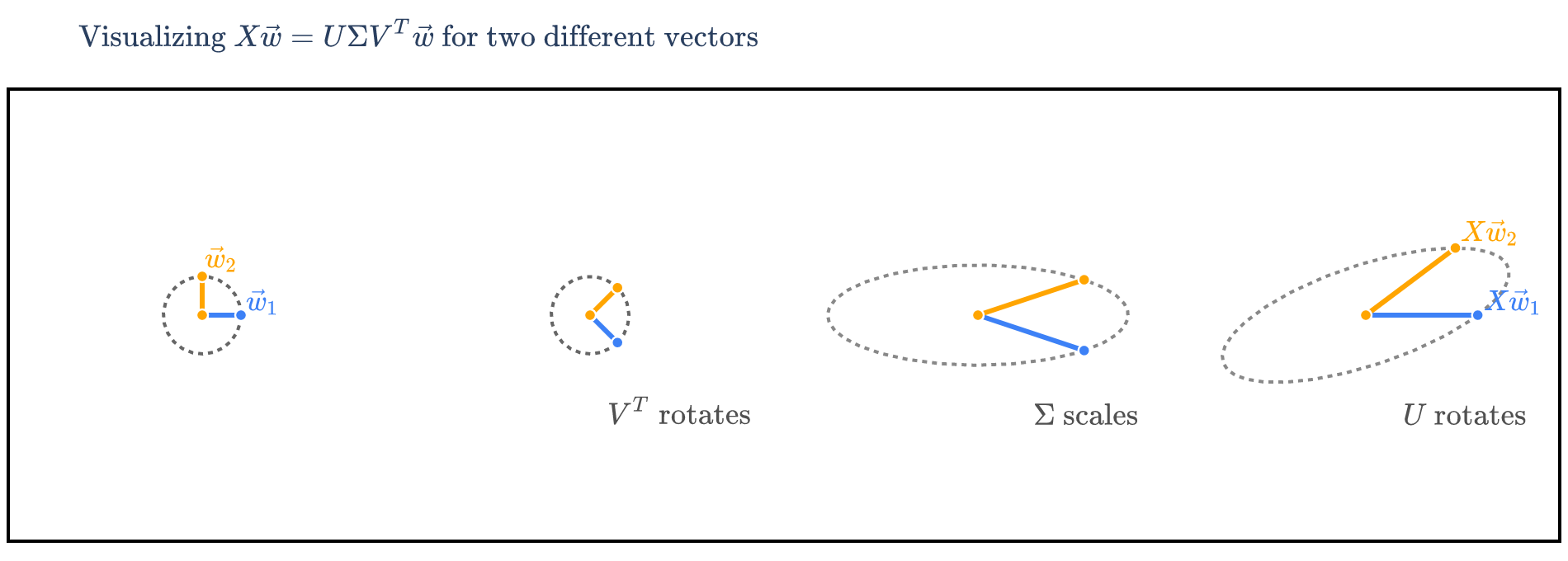
Visualizing the SVD
In Chapter 9.5, we visualized the spectral theorem, which decomposed a symmetric matrix , which we said represented a rotation, stretch, and rotation back.
can be interpreted similarly. If we think of as a linear transformation from to , then operates on in three stages:
a rotation by (because is orthogonal), followed by
a stretch by , followed by
a rotation by
To illustrate, let’s consider the square (but not symmetric) matrix
from one of the earlier worked examples. Unfortunately, it’s difficult to visualize the SVD of matrices larger than , since then either the ’s or ’s (or both) are in or higher.
’s SVD is
In Chapter 10.2, we’ll see how the singular value decomposition can be used to construct low-rank approximations of matrices. A good summary of the SVD is also found at the end of Chapter 10.2.