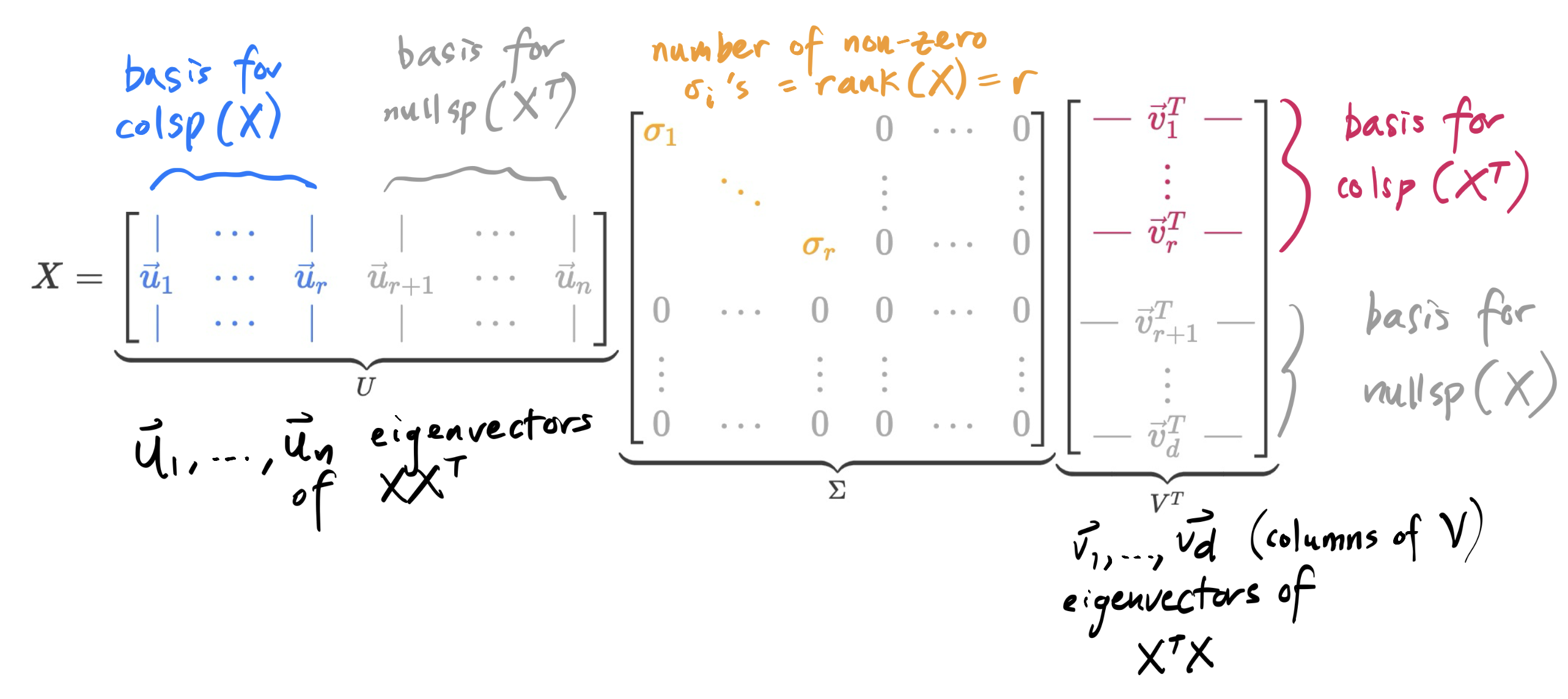
10.2. Low-Rank Approximation - EECS 245 Course Notes

Full SVD¶

The version of the SVD we’ve constructed together is called the full SVD.

In the full SVD, $U$ is $n \times n$ , $\mathcal{\Sigma}$ is $n \times d$ , and $V^T$ is $d \times d$ . If $\text{rank}(X) = r$ , then

The first $r$ columns of $U$ are the left singular vectors of $X$ and are a basis for $\text{colsp}(X)$ ; the last $n - r$ columns of $U$ are a basis for $\text{nullsp}(X^T)$ . Together, the columns of $U$ span $\mathbb{R}^n$ .
The first $r$ columns of $V$ are the right singular vectors of $X$ and are a basis for $\text{colsp}(X^T)$ ; the last $d - r$ columns of $V$ are a basis for $\text{nullsp}(X)$ . Together, the columns of $V$ span $\mathbb{R}^d$ .

The full SVD is nice for proofs, but is a little... annoying to use in real applications, because it contains a lot of 0’s. The additional $n - r$ columns of $U$ and $d - r$ columns of $V$ are included to make $U$ and $V$ orthogonal matrices, but end up getting 0’d out when multiplied by the corresponding 0’s in $\mathcal{\Sigma}$ .

Remember that $X = U \Sigma V^T$ is equivalent to $XV = U \Sigma$ , which says that, for $i = 1, 2, ..., d$ ,

X \vec v_i = \sigma_i \vec u_i

but when $i > r$ , all this says is $\vec 0 = \vec 0$ :

$X \vec v_i = \vec 0$ , since $\vec v_r$ , $\vec v_{r+1}$ , ..., $\vec v_d$ are all in $\text{nullsp}(X)$ , and
$\sigma_i = 0$ , so $\sigma_i \vec u_i = 0 \vec u_i = \vec 0$ .

Compact SVD¶

The compact SVD throws away the 0’s in $\mathcal{\Sigma}$ and the corresponding columns in $U$ and $V$ . In the annotated figure above, it keeps only the first $r$ columns in $\color{#3d81f6} U$ , first r values in $\color{orange} \Sigma$ , and first r rows in $\color{d81a60} V^T$ .

That is, the compact SVD says $X = U_r \Sigma_r V_r^T$ , where $U_r$ is $n \times r$ , $\Sigma_r$ is $r \times r$ , and $V_r^T$ is $r \times d$ .

X = \underbrace{ \begin{bmatrix} {\color{#3d81f6} |} & {\color{#3d81f6} \cdots} & {\color{#3d81f6} |} \\ {\color{#3d81f6} \vec u_1} & {\color{#3d81f6} \cdots} & {\color{#3d81f6} \vec u_r} \\ {\color{#3d81f6} |} & {\color{#3d81f6} \cdots} & {\color{#3d81f6} |} \end{bmatrix} }_{U_r} \underbrace{ \begin{bmatrix} {\color{orange} \sigma_1} & & \\ & {\color{orange} \ddots} & \\ & & {\color{orange} \sigma_r} \end{bmatrix} }_{\Sigma_r} \underbrace{ \begin{bmatrix} {\color{#d81a60}\text{---} \:\: \vec v_1^T \:\: \text{---}} \\ {\color{#d81a60} \vdots} \\ {\color{#d81a60}\text{---} \:\: \vec v_r^T \:\: \text{---}} \end{bmatrix} }_{V_r^T}

The full and compact SVDs are equivalent, in that $X = U \Sigma V^T = U_r \Sigma_r V_r^T$ . But the individual components are of different sizes:

	Full SVD	Compact SVD
$U$	$n \times n$	$n \times r$	First $r$ columns of $U$ are basis for $\text{colsp}(X)$
$\mathcal{\Sigma}$	$n \times d$	$r \times r$	Number of non-zero $\sigma_i$ ’s is $r = \text{rank}(X)$
$V^T$	$d \times d$	$r \times d$	First $r$ rows of $V^T$ are basis for $\text{colsp}(X^T)$

$U_r$ and $V_r$ are no longer orthogonal matrices, since only square matrices can be orthogonal. However, their columns are still orthonormal, meaning $U_r^T U_r = I_{r \times r}$ and $V_r^T V_r = I_{r \times r}$ .

We now compare full vs. compact SVD and use the decomposition for low-rank approximation.

SVD as a Sum¶

The compact SVD hints at another way to think about $X$ .

\begin{align*} X &= \underbrace{ \begin{bmatrix} {\color{#3d81f6} |} & {\color{#3d81f6} \cdots} & {\color{#3d81f6} |} \\ {\color{#3d81f6} \vec u_1} & {\color{#3d81f6} \cdots} & {\color{#3d81f6} \vec u_r} \\ {\color{#3d81f6} |} & {\color{#3d81f6} \cdots} & {\color{#3d81f6} |} \end{bmatrix} }_{U_r} \underbrace{ \begin{bmatrix} {\color{orange} \sigma_1} & & \\ & {\color{orange} \ddots} & \\ & & {\color{orange} \sigma_r} \end{bmatrix} }_{\Sigma_r} \underbrace{ \begin{bmatrix} {\color{#d81a60}\text{---} \:\: \vec v_1^T \:\: \text{---}} \\ {\color{#d81a60} \vdots} \\ {\color{#d81a60}\text{---} \:\: \vec v_r^T \:\: \text{---}} \end{bmatrix} }_{V_r^T} \\ &= \begin{bmatrix} | & \cdots & | \\ {\color{orange} \sigma_1} {\color{#3d81f6} \vec u_1} & \cdots & {\color{orange} \sigma_r} {\color{#3d81f6} \vec u_r} \\ | & \cdots & | \end{bmatrix} \begin{bmatrix} {\color{#d81a60}\text{---} \:\: \vec v_1^T \:\: \text{---}} \\ {\color{#d81a60} \vdots} \\ {\color{#d81a60}\text{---} \:\: \vec v_r^T \:\: \text{---}} \end{bmatrix} \\ &= {\color{orange} \sigma_1} {\color{#3d81f6} \vec u_1} {\color{#d81a60}\vec v_1^T} + {\color{orange} \sigma_2} {\color{#3d81f6} \vec u_2} {\color{#d81a60}\vec v_2^T} + \cdots + {\color{orange} \sigma_r} {\color{#3d81f6} \vec u_r} {\color{#d81a60}\vec v_r^T} \end{align*}

Each term ${\color{orange} \sigma_i} {\color{#3d81f6} \vec u_i} {\color{#d81a60}\vec v_i^T}$ is an outer product of ${\color{#3d81f6} \vec u_i}$ and ${\color{#d81a60}\vec v_i}$ , scaled by ${\color{orange} \sigma_i}$ . Outer products are rank-one matrices: each column of ${\color{orange} \sigma_i} {\color{#3d81f6} \vec u_i} {\color{#d81a60}\vec v_i^T}$ is a multiple of ${\color{#3d81f6} \vec u_i}$ , and each row of it is a multiple of ${\color{#d81a60}\vec v_i^T}$ .

This outer product view of matrix multiplication is not one that we’ve emphasized a ton in this course, but it can be useful in certain contexts, as we’re about to see. To see how it works, let’s revisit our first example.

\underbrace{\begin{bmatrix} 3 & 2 & 5 \\ 2 & 3 & 5 \\ 2 & -2 & 0 \\ 5 & 5 & 10 \end{bmatrix}}_X = \underbrace{\begin{bmatrix} {\color{#3d81f6} \frac{1}{\sqrt{6}}} & {\color{#ff8c00} \frac{1}{3\sqrt{2}}} & {\color{#aaa} -\frac{1}{\sqrt{3}}} & {\color{#aaa} -\frac{2}{3}} \\ {\color{#3d81f6} \frac{1}{\sqrt{6}}} & {\color{#ff8c00} -\frac{1}{3\sqrt{2}}} & {\color{#aaa} -\frac{1}{\sqrt{3}}} & {\color{#aaa} \frac{2}{3}} \\ {\color{#3d81f6} 0} & {\color{#ff8c00} \frac{2\sqrt{2}}{3}} & {\color{#aaa} 0} & {\color{#aaa} \frac{1}{3}} \\ {\color{#3d81f6} \frac{2}{\sqrt{6}}} & {\color{#ff8c00} 0} & {\color{#aaa} \frac{1}{\sqrt{3}}} & {\color{#aaa} 0} \end{bmatrix}}_{U} \underbrace{\begin{bmatrix} {\color{#3d81f6} 15} & {\color{#aaa} 0} & {\color{#aaa} 0} \\ {\color{#aaa} 0} & {\color{#ff8c00} 3} & {\color{#aaa} 0} \\ {\color{#aaa} 0} & {\color{#aaa} 0} & {\color{#aaa} 0} \\ {\color{#aaa} 0} & {\color{#aaa} 0} & {\color{#aaa} 0} \end{bmatrix}}_{\Sigma} \underbrace{\begin{bmatrix} {\color{#3d81f6} \frac{1}{\sqrt{6}}} & {\color{#3d81f6} \frac{1}{\sqrt{6}}} & {\color{#3d81f6} \frac{2}{\sqrt{6}}} \\ {\color{#ff8c00} \frac{1}{\sqrt{2}}} & {\color{#ff8c00} -\frac{1}{\sqrt{2}}} & {\color{#ff8c00} 0} \\ {\color{#aaa} \frac{1}{\sqrt{3}}} & {\color{#aaa} \frac{1}{\sqrt{3}}} & {\color{#aaa} -\frac{1}{\sqrt{3}}} \end{bmatrix}}_{V^T}

The summation view of the SVD says that:

\begin{align*} X =\;& {\color{#3d81f6} 15} \begin{bmatrix} {\color{#3d81f6} \frac{1}{\sqrt{6}}} \\ {\color{#3d81f6} \frac{1}{\sqrt{6}}} \\ {\color{#3d81f6} 0} \\ {\color{#3d81f6} \frac{2}{\sqrt{6}}} \end{bmatrix} \begin{bmatrix} {\color{#3d81f6} \frac{1}{\sqrt{6}}} & {\color{#3d81f6} \frac{1}{\sqrt{6}}} & {\color{#3d81f6} \frac{2}{\sqrt{6}}} \end{bmatrix} + {\color{#ff8c00} 3} \begin{bmatrix} {\color{#ff8c00} \frac{1}{3\sqrt{2}}} \\ {\color{#ff8c00} -\frac{1}{3\sqrt{2}}} \\ {\color{#ff8c00} \frac{2\sqrt{2}}{3}} \\ {\color{#ff8c00} 0} \end{bmatrix} \begin{bmatrix} {\color{#ff8c00} \frac{1}{\sqrt{2}}} & {\color{#ff8c00} -\frac{1}{\sqrt{2}}} & {\color{#ff8c00} 0} \end{bmatrix} \\ &= \underbrace{{\color{#3d81f6} \begin{bmatrix} \frac{5}{2} & \frac{5}{2} & 5 \\ \frac{5}{2} & \frac{5}{2} & 5 \\ 0 & 0 & 0 \\ 5 & 5 & 10 \end{bmatrix}}}_{\text{rank-one matrix}} + \underbrace{{\color{orange} \begin{bmatrix} \frac{1}{2} & -\frac{1}{2} & 0 \\ -\frac{1}{2} & \frac{1}{2} & 0 \\ 2 & -2 & 0 \\ 0 & 0 & 0 \end{bmatrix}}}_{\text{rank-one matrix}} \end{align*}

Since ${\color{#3d81f6} 15} > {\color{orange} 3}$ , the first outer product contributes more to $X$ than the second one does.

We can think of the singular values as representing the importance of the corresponding singular vectors in representing $X$ . Since we sort singular values in decreasing order, $\sigma_1 \geq \sigma_2 \geq ... \geq \sigma_r > 0$ , the first outer product is always the most important one, the second outer product is the second most important one, and so on.

Low-Rank Approximation¶

Our most recent observation is that the SVD $X = U \Sigma V^T$ allows us to write $X$ as a sum of rank-one matrices, in decreasing order of importance.

X = \underbrace{\sigma_1 \vec u_1 \vec v_1^T}_{\text{most important}} + \underbrace{\sigma_2 \vec u_2 \vec v_2^T}_{\text{second most important}} + \cdots + \underbrace{\sigma_r \vec u_r \vec v_r^T}_{\text{least important}}

In many practical applications, the full matrix $X$ can be too large to store or process. In such cases, we can produce a low-rank approximation of $X$ by summing fewer than $r$ of these rank-one matrices. In the example above, $X$ was of rank 2, so a rank-1 approximation of $X$ would just be the first outer product, $\sigma_1 \vec u_1 \vec v_1^T$ , which is in blue above.

Example: Image Compression¶

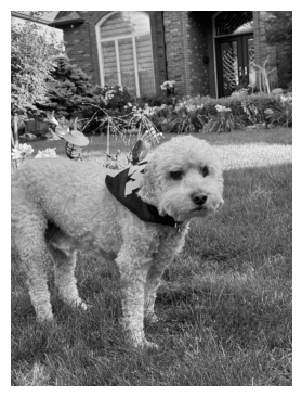
A common application of the SVD and low-rank approximations is to compress images. How so? Consider the following grayscale image of my (16 year old) dog, Junior.

import numpy as np
import matplotlib.pyplot as plt
from PIL import Image

# Load the image and convert to grayscale
img = Image.open('imgs/junior.jpeg').convert('L')
img_arr = np.rot90(np.array(img), k=3)

# Show the grayscale image
plt.figure(figsize=(4*1.5, 3*1.5))
plt.imshow(img_arr, cmap='gray')
plt.axis('off')
plt.show()

This image is 300 pixels wide and 400 pixels tall. Since the image is grayscale, each pixel’s intensity can be represented by a number between 0 and 255, where 0 is black and 255 is white. These intensities can be stored in a $400 \times 300$ matrix. The rank of this matrix is likely 300, since it’s extremely unlikely that any of the 300 columns of the image are exactly representable as a linear combination of other columns.

But, as the SVD reveals, the image can be approximated well by a rank- $k$ matrix, for a $k$ that is much smaller than 300. We build this low-rank approximation of the image by summing up $k$ rank-one matrices.

\text{rank } k \text{ approximation of image} = \sum_{i=1}^k \sigma_i \vec u_i \vec v_i^T

A slider should appear below, allowing you to select a value of $k$ and see the corresponding rank- $k$ approximation of Junior.

import numpy as np
import plotly.graph_objs as go
from PIL import Image

IMAGE_PATH = 'imgs/junior.jpeg'

# Load image (fallback to dummy if not found), rotate 90º clockwise, and resize to 3:4 aspect ratio (e.g., 300x400)
try:
    img = Image.open(IMAGE_PATH).convert('L')
    img = img.rotate(-90, expand=True)  # Rotate 90º clockwise
    img = img.resize((300, 400), Image.LANCZOS)  # 3:4 aspect ratio (width, height)
    img_arr = np.array(img)
except FileNotFoundError:
    H, W = 400, 300  # 3:4 aspect ratio
    img_arr = np.zeros((H, W), dtype=np.uint8)
    for i in range(H):
        for j in range(W):
            img_arr[i, j] = 200 if ((i // 10) % 2 == (j // 10) % 2) else 50

# Compute SVD
U, S, VT = np.linalg.svd(img_arr.astype(float), full_matrices=False)
max_k = len(S)

def get_reconstruction(k):
    k = max(1, min(k, len(S)))
    Uk = U[:, :k]
    Sk = S[:k]
    VTk = VT[:k, :]
    recon = Uk @ np.diag(Sk) @ VTk
    return 255 - np.clip(recon, 0, 255).astype(np.uint8)

# k=1, k=31, k=61, k=91, ..., max allowed (up to len(S))
ks = list(range(1, 51))
if ks[-1] != max_k-1:
    ks.append(max_k)

# Create frames (each frame is a Heatmap of the reconstructed image)
frames = []
for k in ks:
    z = get_reconstruction(k)
    frames.append(
        go.Frame(
            data=[
                go.Heatmap(
                    z=z,
                    zmin=0,
                    zmax=255,
                    colorscale=[[0, "white"], [1, "black"]],
                    showscale=False
                )
            ],
            name=str(k)
        )
    )

# Initial trace uses k=1
initial_z = get_reconstruction(1)
initial_trace = go.Heatmap(z=initial_z, zmin=0, zmax=255, colorscale=[[0, "white"], [1, "black"]], showscale=False)

fig = go.Figure(
    data=[initial_trace],
    frames=frames
)

# Slider that calls animate on each frame
slider_steps = []
for k in ks:
    step = {
        "args": [
            [str(k)],  # frame name
            {
                "frame": {"duration": 0, "redraw": True},
                "mode": "immediate",
                "transition": {"duration": 0}
            }
        ],
        "label": str(k),
        "method": "animate"
    }
    slider_steps.append(step)

sliders = [{
    "active": 0,
    "pad": {"t": 50},
    "steps": slider_steps,
    "currentvalue": {"prefix": "Rank k: ", "font": {"size": 14}}
}]

fig.update_layout(
    sliders=sliders,
    width=300,   # width matches aspect ratio
    height=480,  # height matches aspect ratio
    margin=dict(l=20, r=20, t=0, b=0),
    font=dict(family="Avenir"),
)

# Hide axes
fig.update_xaxes(visible=False)
fig.update_yaxes(visible=False)
fig.update_yaxes(autorange="reversed")

fig.show()

To store the full image, we need to store $400 \cdot 300 = 120{,}000$ numbers. But to store a rank- $k$ approximation of the image, we only need to store $(1 + 400 + 300)k = 701k$ numbers – only the first $k$ singular values, along with $\vec u_1, \vec u_2, ..., \vec u_k$ (each of which has 400 numbers), and $\vec v_1, \vec v_2, ..., \vec v_k$ (each of which has 300 numbers). If we’re satisfied with a rank-30 approximation, we only need to store $701 \cdot 30 = 21{,}030$ numbers, which is a compression of $\frac{120{,}000}{21{,}030} \approx 5.7$ times!

Computing the SVD¶

Finally, I’ll show you how to use numpy to compute the SVD of a matrix. The key function is np.linalg.svd. Let’s apply it to our familiar example,

\underbrace{\begin{bmatrix} 3 & 2 & 5 \\ 2 & 3 & 5 \\ 2 & -2 & 0 \\ 5 & 5 & 10 \end{bmatrix}}_X = \underbrace{\begin{bmatrix} \frac{1}{\sqrt{6}} & \frac{1}{3\sqrt{2}} & -\frac{1}{\sqrt{3}} & -\frac{2}{3} \\ \frac{1}{\sqrt{6}} & -\frac{1}{3\sqrt{2}} & -\frac{1}{\sqrt{3}} & \frac{2}{3} \\ 0 & \frac{2\sqrt{2}}{3} & 0 & \frac{1}{3} \\ \frac{2}{\sqrt{6}} & 0 & \frac{1}{\sqrt{3}} & 0 \end{bmatrix}}_{U} \underbrace{\begin{bmatrix} 15 & 0 & 0 \\ 0 & 3 & 0 \\ 0 & 0 & 0 \\ 0 & 0 & 0 \end{bmatrix}}_{\Sigma} \underbrace{\begin{bmatrix} \frac{1}{\sqrt{6}} & \frac{1}{\sqrt{6}} & \frac{2}{\sqrt{6}} \\ \frac{1}{\sqrt{2}} & -\frac{1}{\sqrt{2}} & 0 \\ \frac{1}{\sqrt{3}} & \frac{1}{\sqrt{3}} & -\frac{1}{\sqrt{3}} \end{bmatrix}}_{V^T}

X = np.array([[3, 2, 5],
              [2, 3, 5],
              [2, -2, 0],
              [5, 5, 10]])
              
u, s, vt = np.linalg.svd(X)
u.shape, s.shape, vt.shape

((4, 4), (3,), (3, 3))

By default, it computes the full SVD, which is why u is of shape $4 \times 4$ and vt is of shape $3 \times 3$ , even though $\text{rank}(X) = 2$ .

s is returned as a 1-dimensional array of singular values.

array([15., 3., 0.])

If we’d like to use u, s, and vt to reconstruct $X$ , we need to reshape s into a matrix with the same shape as $X$ .

ss = np.zeros(X.shape)
ss[np.arange(len(s)), np.arange(len(s))] = s
ss

array([[15.,  0.,  0.],
       [ 0.,  3.,  0.],
       [ 0.,  0.,  0.],
       [ 0.,  0.,  0.]])

u @ ss @ vt

array([[ 3.,  2.,  5.],
       [ 2.,  3.,  5.],
       [ 2., -2.,  0.],
       [ 5.,  5., 10.]])

Notice: The signs of the columns of $U$ and $V$ are not uniquely determined by the SVD. For example, we could replace $\vec u_1$ with $-\vec u_1$ and $\vec v_1$ with $-\vec v_1$ to get the same matrix $X$ . The values for $U$ we found had flipped signs for columns 1, 2 relative to the values returned by np.linalg.svd.

\text{our } U = \begin{bmatrix} \frac{1}{\sqrt{6}} & \frac{1}{3\sqrt{2}} & -\frac{1}{\sqrt{3}} & -\frac{2}{3} \\ \frac{1}{\sqrt{6}} & -\frac{1}{3\sqrt{2}} & -\frac{1}{\sqrt{3}} & \frac{2}{3} \\ 0 & \frac{2\sqrt{2}}{3} & 0 & \frac{1}{3} \\ \frac{2}{\sqrt{6}} & 0 & \frac{1}{\sqrt{3}} & 0 \end{bmatrix}

np.set_printoptions(precision=8, suppress=True)

array([[-0.40824829,  0.23570226, -0.45735398, -0.75405909],
       [-0.40824829, -0.23570226, -0.68098866,  0.56038577],
       [-0.        ,  0.94280904, -0.05590867,  0.32861122],
       [-0.81649658, -0.        ,  0.56917132,  0.09683666]])

The first column of numpy’s u is the negative of our first column of $U$ .
Both second columns are the same.
The latter two columns are different. Why? There are infinitely many orthogonal bases for the null space of $X^T$ , which are what the last two columns of $U$ represent. We just picked a different choice than numpy did.

Key Takeaways¶

To recap:

All $n \times d$ matrices $X$ have a singular value decomposition $X = U \Sigma V^T$ , where $U$ is $n \times n$ , $\mathcal{\Sigma}$ is $n \times d$ , and $V$ is $d \times d$ .

The columns of $U$ are orthonormal eigenvectors of $XX^T$ ; these are called the left singular vectors of $X$ .
The columns of $V$ are orthonormal eigenvectors of $X^TX$ ; these are called the right singular vectors of $X$ .
Both $XX^T$ and $X^TX$ share the same non-zero eigenvalues; the singular values of $X$ are the square roots of these eigenvalues. The number of non-zero singular values is equal to the rank of $X$ . It’s important that we sort the singular values in decreasing order, so that $\sigma_1 \geq \sigma_2 \geq ... \geq \sigma_r > 0$ , and place the singular vectors in the columns of $U$ and $V$ in the same order.
$\sigma_i = \sqrt{\lambda_i}$
A typical recipe for computing the SVD is to:
1. Compute $X^TX$ . Place its eigenvectors in the columns of $V$ , and place the square roots of its eigenvalues in the diagonal of $\mathcal{\Sigma}$ .
2. To find each $\vec u_i$ , use $X \vec v_i = \sigma_i \vec u_i$ , i.e. $\vec u_i = \frac{1}{\sigma_i} X \vec v_i$ .
3. The above rule only works for $\sigma_i > 0$ . If $\sigma_i = 0$ , then the remaining $\vec u_i$ ’s must be eigenvectors of $XX^T$ for the eigenvalue 0, meaning they must lie in the nullspace of $X^T$ .
The SVD allows us to interpret the linear transformation of multiplying by $X$ as a composition of a rotation by $V^T$ , a scaling/stretching by $\mathcal{\Sigma}$ , and a rotation by $U$ .
The SVD $X = U \Sigma V^T$ can be viewed as a sum of rank-one matrices:
$X = \sum_{i=1}^r \sigma_i \vec u_i \vec v_i^T$
Each piece $\sigma_i \vec u_i \vec v_i^T$ is a rank-one matrix, consisting of the outer product of $\vec u_i$ and $\vec v_i$ . This summation view can be used to compute a low-rank approximation of $X$ by summing fewer than $r$ of these rank-one matrices.
$X_k = \sum_{i=1}^k \sigma_i \vec u_i \vec v_i^T$