5.2. Transpose and Special Matrices - EECS 245 Course Notes

There’s an important operation on matrices that we haven’t discussed yet. Let me introduce it, and then walk through a few types of matrices that are important enough to be given names.

Transpose¶

To illustrate, let’s start with our familiar matrix $A$ :

A = \begin{bmatrix} 3 & {\color{#3d81f6} \mathbf{1}} & 4 \\ 2 & {\color{#3d81f6} \mathbf{1}} & 9 \\ 0 & {\color{#3d81f6} \mathbf{-1}} & 0 \\ 2 & {\color{#3d81f6} \mathbf{-2}} & 0 \end{bmatrix}

The transpose of $A$ is:

A^T = \begin{bmatrix} 3 & 2 & 0 & 2 \\ {\color{#3d81f6} \mathbf{1}} & {\color{#3d81f6} \mathbf{1}} & {\color{#3d81f6} \mathbf{-1}} & {\color{#3d81f6} \mathbf{-2}} \\ 4 & 9 & 0 & 0 \end{bmatrix}

Note that $A \in \mathbb{R}^{4 \times 3}$ and $A^T \in \mathbb{R}^{3 \times 4}$ .

Why would we ever need to do this? To illustrate, suppose $\vec u = \begin{bmatrix} u_1 \\ u_2 \\ u_3 \\ u_4 \end{bmatrix}$ , and that we’d like to compute the product $A^T \vec u$ . (Note that $\vec u$ must be in $\mathbb{R}^4$ in order for $A^T \vec u$ to be defined, unlike $\vec x \in \mathbb{R}^3$ in the product $A \vec x$ ). Then:

\begin{align*}A^T \vec u &= \begin{bmatrix} 3 & 2 & 0 & 2 \\ 1 & 1 & -1 & -2 \\ 4 & 9 & 0 & 0 \end{bmatrix} \begin{bmatrix} {\color{orange} \mathbf{u_1}} \\ {\color{orange} \mathbf{u_2}} \\ {\color{orange} \mathbf{u_3}} \\ {\color{orange} \mathbf{u_4}} \end{bmatrix} \\ &= {\color{orange} \mathbf{u_1}} \begin{bmatrix} 3 \\ 1 \\ 4 \end{bmatrix} + {\color{orange} \mathbf{u_2}} \begin{bmatrix} 2 \\ 1 \\ 9 \end{bmatrix} + {\color{orange} \mathbf{u_3}} \begin{bmatrix} 0 \\ -1 \\ 0 \end{bmatrix} + {\color{orange} \mathbf{u_4}} \begin{bmatrix} 2 \\ -2 \\ 0 \end{bmatrix} \end{align*}

This is a linear combination of the rows of $A$ , where the weights are the components of $\vec u$ . Remember, the standard product $A \vec x$ is a linear combination of the columns of $A$ , so the transpose helps us if we want to compute a linear combination of the rows of $A$ . (Equivalently, it helps us if we want to compute the dot product of the columns of $A$ with $\vec u$ – see the linear combination interpretation section of Chapter 5.1.)

The transpose also gives us another way of expressing the dot product of two vectors. If $\color{orange} \vec u$ and $\color{#3d81f6} \vec v$ are two vectors in $\mathbb{R}^n$ , then $\color{orange} \vec u^T$ is a row vector with 1 row and $n$ columns. Multiplying $\color{orange} \vec u^T$ by $\color{#3d81f6} \vec v$ results in a $1 \times 1$ matrix, which is just the scalar ${\color{orange} \vec u} \cdot {\color{#3d81f6} \vec v}$ .

\vec {\color{orange}u}^T \vec{\color{#3d81f6}v} = \begin{bmatrix} {\color{orange}u_1} & {\color{orange}u_2} & \ldots & {\color{orange}u_n} \end{bmatrix} \begin{bmatrix}{\color{#3d81f6}v_1} \\{\color{#3d81f6}v_2} \\ \vdots \\{\color{#3d81f6}v_n} \end{bmatrix} = {\color{orange}u_1}{\color{#3d81f6}v_1} + {\color{orange}u_2}{\color{#3d81f6}v_2} + \ldots + {\color{orange}u_n}{\color{#3d81f6}v_n} = \vec {\color{orange}u} \cdot \vec{\color{#3d81f6}v} = \vec{\color{#3d81f6}v} \cdot \vec {\color{orange}u} = \vec{\color{#3d81f6}v}^T \vec {\color{orange}u}

The benefit of using the transpose to express the dot product is that it allows us to write the dot product of two vectors in terms of matrix multiplication, rather than being an entirely different type of operation. (In fact, as we’ve seen here, matrix multiplication is just a generalization of the dot product.)

There are other uses for the transpose, too, so it’s a useful tool to have in your toolbox.

Properties¶

The first three properties are relatively straightforward. The last property is a bit more subtle. Try and reason as to why it’s true on your own, then peek into the box below to verify your reasoning and to see an example.

Why is

(AB)^T = B^T A^T

Let’s start with just $(AB)^T$ and reason our way from there. Define $C = (AB)^T$ . $C$ is presumably the product of two matrices $X$ and $Y$ , we just don’t know what $X$ and $Y$ are. By the definition of matrix multiplication, we know that $C_{ij}$ is the dot product of the $i$ th row of $X$ and the $j$ th column of $Y$ . How can we express the product $C = XY$ in terms of $A$ and $B$ ?

Let’s work backwards. Since $C_{ij} = (AB)^T_{ij} = (AB)_{ji}$ by the definition of the transpose, we know that:

C_{ij} = (AB)_{ji} = \left( \text{row } j \text{ of } A \right) \cdot \left( \text{column } i \text{ of } B \right) = \left( \text{column } i \text{ of } B \right) \cdot \left( \text{row } j \text{ of } A \right)

This is a little backwards relative to the definition of matrix multiplication, which says that:

C_{ij} = (XY)_{ij} = \left( \text{row } i \text{ of } X \right) \cdot \left( \text{column } j \text{ of } Y \right)

In order for the two definitions of $C_{ij}$ to be consistent, we must have:

\left( \text{column } i \text{ of } B \right) \cdot \left( \text{row } j \text{ of } A \right) = \left( \text{row } i \text{ of } X \right) \cdot \left( \text{column } j \text{ of } Y \right)

Row $i$ of $X$ is the same as column $i$ of $B$ , if $X = B^T$ .
Column $j$ of $Y$ is the same as row $j$ of $A$ , if $Y = A^T$ .

Putting this together, we have:

C = (AB)^T = B^T A^T

as we hoped!

To make things concrete, let’s consider two new matrices $A$ and $B$ :

A = \begin{bmatrix} 0 & -1 \\ 4 & 2 \\ 3 & 9 \\ 0 & 1 \end{bmatrix} \quad B = \begin{bmatrix} 1 & 2 & 3 \\ -1 & -2 & 4 \end{bmatrix}

Then,

AB = \begin{bmatrix} 0 & -1 \\ 4 & 2 \\ {\color{#3d81f6} \mathbf{3}} & {\color{#3d81f6} \mathbf{9}} \\ 0 & 1 \end{bmatrix} \begin{bmatrix} 1 & 2 & {\color{#3d81f6} \mathbf{3}} \\ -1 & -2 & {\color{#3d81f6} \mathbf{4}} \end{bmatrix} = \begin{bmatrix} 1 & 2 & -4 \\ 2 & 4 & 20 \\ -6 & -12 & \boxed{{\color{#3d81f6} \mathbf{45}}} \\ -1 & -2 & 4 \end{bmatrix}

And:

B^T A^T = \begin{bmatrix} 1 & -1 \\ 2 & -2 \\ {\color{#3d81f6} \mathbf{3}} & {\color{#3d81f6} \mathbf{4}} \end{bmatrix} \begin{bmatrix} 0 & 4 & {\color{#3d81f6} \mathbf{3}} & 0 \\ -1 & 2 & {\color{#3d81f6} \mathbf{9}} & 1 \end{bmatrix} = \begin{bmatrix} 1 & 2 & -6 & -1 \\ 2 & 4 & -12 & -2 \\ -4 & 20 & \boxed{{\color{#3d81f6} \mathbf{45}}} & 4 \end{bmatrix}

$B^T A^T$ is the transpose of $AB$ . Both $AB$ and $B^T A^T$ have 12 elements, both computed using the same 12 dot products.

The fact that $(AB)^T = B^T A^T$ comes in handy when finding the norm of a matrix-vector product. If $A$ is an $n \times d$ matrix and $\vec x \in \mathbb{R}^d$ , then:

\lVert A \vec x \rVert^2 = (A \vec x)^T (A \vec x) = \vec x^T A^T A \vec x

As we’ll soon see, some matrices $A$ have special properties that make this computation particularly easy.

In numpy, the T attribute is used to compute the transpose of a 2D array.

Activity 1¶

Activity 1

Activity 1.1

In the cell above:

Define x to be an array corresponding to the vector $\vec x = \begin{bmatrix} 1 \\ 0 \\ 3 \end{bmatrix}$ .
Find the norm of the product $A \vec x$ using np.linalg.norm.
Find the norm of the product $A \vec x$ using the fact that $\lVert A \vec x \rVert^2 = \vec x^T A^T A \vec x$ , and verify that you get the same answer.

Activity 1.2

Suppose $M \in \mathbb{R}^{n \times d}$ is a matrix, $\vec{v} \in \mathbb{R}^d$ is a vector, and $s \in \mathbb{R}$ is a scalar.

Determine whether each of the following quantities is a matrix, vector, scalar, or undefined. If the result is a matrix or vector, determine its dimensions.

$M\vec{v}$
$\vec{v} M$
$\vec{v}^2$
$M^TM$
$MM^T$
$\vec{v}^T M \vec{v}$
$(sM\vec{v}) \cdot (sM\vec{v})$
$(s \vec{v}^T M^T)^T$
$\vec{v}^T M^T M \vec{v}$
$\vec{v}\vec{v}^T + M^TM$
$\frac{M \vec{v}}{\lVert \vec{v} \rVert} + (\vec{v}^T M^T M \vec{v}) M \vec{v}$

Activity 1.3

Let $A = \begin{bmatrix} 2 & 1 \\ 3 & 4 \\ -1 & 1 \end{bmatrix}$ , $B = \begin{bmatrix} 1 & 0 & 2 \\ 2 & 1 & 3 \end{bmatrix}$ , and $C = \begin{bmatrix} 1 & 0 & 2 & -1 \\ 0 & 1 & 1 & 1 \\ 1 & 1 & 0 & -1 \end{bmatrix}$ .

Compute $AB$ , then multiply the result by $C$ .
Compute $A$ , then multiply the result by $BC$ . Do you get the same result as above? If so, what property of matrix multiplication guarantees this?
Determine a formula for $(ABC)^T$ , and verify that your result works. (Hint: Start with the fact that $(AB)^T = B^T A^T$ .)

The Identity Matrix¶

Now, I’ll introduce several “special” types of matrices that will come in handy at various points throughout our journey.

Saying “the identity matrix” is a bit ambiguous, as there are infinitely many identity matrices – there’s a $1 \times 1$ identity matrix, a $2 \times 2$ identity matrix, a $3 \times 3$ identity matrix, and so on. Often, the dimension of the identity matrix is implied by context, and if not, we might provide it as a subscript, e.g. $I_n$ for the $n \times n$ identity matrix.

Why is the identity matrix defined this way? It’s the matrix equivalent of the number 1 in scalar multiplication, also known as the multiplicative identity. If $c$ is a scalar, then $c \cdot 1 = c$ and $1 \cdot c = c$ . (0 is known as the additive identity in scalar multiplication.)

Similarly, if $A$ is square $n \times n$ matrix and $\vec x \in \mathbb{R}^n$ is a vector, then the $n \times n$ identity matrix $I$ is the unique matrix that satisfies:

$I \vec x = \vec x$ for all $\vec x \in \mathbb{R}^n$ .
$I A = A I = A$ for all $A \in \mathbb{R}^{n \times n}$ .

A good exercise is to verify that the identity matrix satisfies these properties.

Activity 2¶

Activity 2

Let $X = \begin{bmatrix} 1 & -2 \\ -1 & 3 \\ 2 & 0 \\ 0 & -1 \\ 3 & 2 \end{bmatrix}$ .

Compute $X^TX$ .
Then, compute the transpose of $X^TX$ . What do you notice? ( $X^TX$ is called a symmetric matrix, as we’ll discuss below.)
Compute $X^TX + \frac{1}{2} I$ .

Symmetric Matrices¶

For example, $A$ below is symmetric, but $B$ is not.

\underbrace{A = \begin{bmatrix} 1 & 4 \\ 4 & 3 \end{bmatrix}, \qquad A^T = \begin{bmatrix} 1 & 4 \\ 4 & 3 \end{bmatrix} = A}_{\text{symmetric}}

\underbrace{B = \begin{bmatrix} 1 & 4 \\ -2 & 3 \end{bmatrix}, \qquad B^T = \begin{bmatrix} 1 & -2 \\ 4 & 3 \end{bmatrix} \neq B}_{\text{not symmetric}}

A symmetric matrix is such that row 1 is the same as column 1, row 2 is the same as column 2, and so on. We’ll see several applications of symmetric matrices later in the course – for example, they are easy to work with in multivariate calculus.

But, where do they come from? Data usually isn’t symmetric: if $X$ is a matrix in which each row is a data point and each column is a feature, then usually $X$ is very tall, and thus can’t be symmetric.

Here’s the key: for any $n \times d$ matrix $X$ , $X^TX$ is a symmetric $d \times d$ matrix.We can verify this using the fact that $(AB)^T = B^T A^T$ .

({\color{orange}X^T}{\color{#3d81f6}X})^T = {\color{#3d81f6}X}^T({\color{orange}X^T})^T = X^TX

I think of $X^TX$ as the dot product matrix of $X$ , because its entries are the dot products of the pairs of columns of $X$ . For example, let

X = \begin{bmatrix} 2 & -6 & 1 \\ 3 & 1 & -1 \end{bmatrix}

Then,

X^TX = \begin{bmatrix} 2 & 3 \\ -6 & 1 \\ 1 & -1 \end{bmatrix} \begin{bmatrix} 2 & -6 & 1 \\ 3 & 1 & -1 \end{bmatrix} = \begin{bmatrix} 13 & -9 & -1 \\ -9 & 37 & -7 \\ -1 & -7 & 2 \end{bmatrix}

$X^TX$ contains the dot products of the columns of $X$ with each other. For instance, -9 in position $(1, 2)$ is the dot product of

row 1 of $X^T$ , which is column 1 of $X$ , with
column 2 of $X$

The elements along the diagonal of $X^TX$ – 13, 37, and 2 – are the dot products of the columns of $X$ with themselves, meaning they are the squared norms of the columns.

Activity 3¶

Activity 3

Above, we defined $X^TX$ as the dot product matrix, since it contained the dot products of the columns of $X$ with each other.

Now, let’s consider $XX^T$ .

What is the shape of $XX^T$ , i.e. how many rows and columns does it have?
What is the English meaning of $XX^T$ ?

Diagonal Matrices¶

Usually, diagonal matrices are square, like the examples below.

\begin{bmatrix} 1 & 0 \\ 0 & 1 \end{bmatrix}, \quad \begin{bmatrix} 2 & 0 \\ 0 & 3 \end{bmatrix}, \quad \begin{bmatrix} -\pi & 0 & 0 \\ 0 & 15 & 0 \\ 0 & 0 & 3 \end{bmatrix}

Notice that the diagonal is down and to the right – position (1, 1) is the first diagonal element, position (2, 2) is the second diagonal element, and so on.

Diagonal matrices don’t have to be square. We could also call the following a diagonal matrix.

\begin{bmatrix} 1 & 0 & 0 \\ 0 & 2 & 0 \end{bmatrix}

What is their significance? Let’s observe what happens when we multiply a diagonal matrix by a vector, as we did in Activity 4. of Chapter 5.1.

\underbrace{\begin{bmatrix} -3 & 0 & 0 \\ 0 & \pi & 0 \\ 0 & 0 & 5 \end{bmatrix}}_{D} \underbrace{\begin{bmatrix} 1 \\ 2 \\ 3 \end{bmatrix}}_{\vec x} = \begin{bmatrix} -3 \\ 2\pi \\ 15 \end{bmatrix}

What happened to $\vec x$ after being multiplied by $D$ ? Each component was stretched. Element 1 of $\vec x$ was stretched by -3, element 2 was stretched by $\pi$ , and element 3 was stretched by 5. The 0’s in the off-diagonal elements allowed $D$ to scale each component of $\vec x$ independently.

Triangular Matrices¶

For instance, $\begin{bmatrix} 1 & 2 & 3 \\ 0 & 4 & 5 \\ 0 & 0 & 6 \end{bmatrix}$ is upper triangular, and $\begin{bmatrix} 1 & 0 & 0 \\ 2 & 3 & 0 \\ 4 & 5 & 6 \end{bmatrix}$ is lower triangular. I’ll have more to say on these matrices later in the term; for now, I just want you to be aware of their existence.

Orthogonal Matrices¶

The final category of matrix I want to introduce here is the orthogonal matrix. It’s the first type of matrix here whose defining property can’t be determined just by looking at the individual elements of the matrix; it involves some computation.

Let’s consider the matrix

A = \begin{bmatrix} \frac{\sqrt{3}}{2} & -\frac{1}{2} \\[6pt] \frac{1}{2} & \frac{\sqrt{3}}{2} \end{bmatrix}

It is orthogonal, because $A^TA$ and $AA^T$ are both equal to the $2 \times 2$ identity matrix. What does this really tell us? When I discussed symmetric matrices above, I said that $A^TA$ for any matrix $A$ contains the dot products of the columns of $A$ with each other. So, if

A^TA = \begin{bmatrix} \frac{\sqrt{3}}{2} & \frac{1}{2} \\[6pt] -\frac{1}{2} & \frac{\sqrt{3}}{2} \end{bmatrix} \begin{bmatrix} \frac{\sqrt{3}}{2} & -\frac{1}{2} \\[6pt] \frac{1}{2} & \frac{\sqrt{3}}{2} \end{bmatrix} = \begin{bmatrix} 1 & 0 \\[6pt] 0 & 1 \end{bmatrix}

this tells us that $A$ ’s columns are:

unit vectors, since the dot product of each column with itself is 1
orthogonal, since the dot product of each column with every other column is 0

Since $AA^T = I$ , too, this means that $A$ ’s rows are also unit vectors that are orthogonal to each other.

So, orthogonal matrices are matrices whose

columns are unit vectors
rows are unit vectors
columns are orthogonal to each other
rows are orthogonal to each other

If a collection of vectors are all unit vectors and orthogonal, we may call that collection orthonormal. So, an orthogonal matrix has orthonormal columns and orthonormal rows.

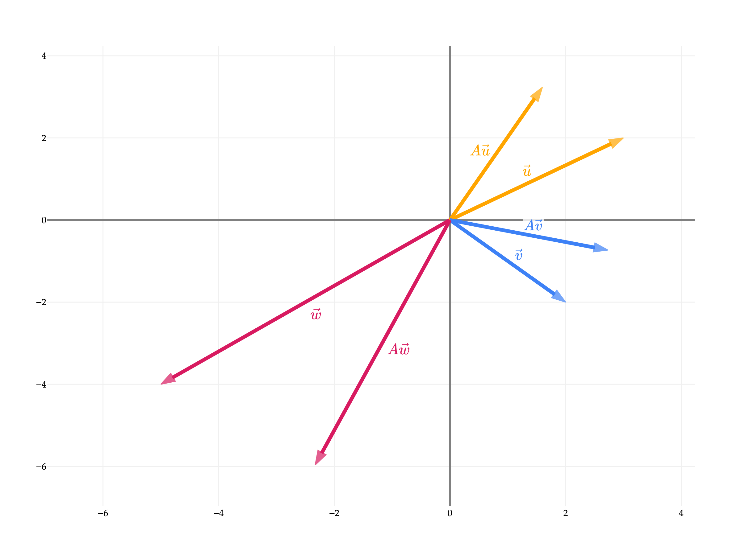
Let’s preview some ideas from Chapter 6.1, let’s visualize six vectors in $\mathbb{R}^2$ .

$\color{orange} \vec u = \begin{bmatrix} 3 \\ 2 \end{bmatrix}$ and $A \color{orange} \vec u$
$\color{#3d81f6} \vec v = \begin{bmatrix} 2 \\ -2 \end{bmatrix}$ and $A \color{#3d81f6} \vec v$
$\color{#d81a60} \vec w = \begin{bmatrix} -5 \\ -4 \end{bmatrix}$ and $A \color{#d81a60} \vec w$

What do you notice about the vectors $A \color{orange} \vec u$ , $A \color{#3d81f6} \vec v$ , and $A \color{#d81a60} \vec w$ ? and how they relate to $\color{orange} \vec u$ , $\color{#3d81f6} \vec v$ , and $\color{#d81a60} \vec w$ ?

from utils import plot_vectors
import numpy as np

A = np.array([[np.cos(np.pi/6), -np.sin(np.pi/6)], [np.sin(np.pi/6), np.cos(np.pi/6)]])
u = np.array([3, 2])
v = np.array([2, -2])
w = np.array([-5, -4])

Au = A @ u
Av = A @ v
Aw = A @ w

fig = plot_vectors([(tuple(u), 'orange', r'$\vec u$'),
              (tuple(v), '#3d81f6', r'$\vec v$'),
              (tuple(w), '#d81a60', r'$\vec w$'),
              (tuple(Au), 'orange', r'$A \vec u$'),
              (tuple(Av), '#3d81f6', r'$A \vec v$'),
              (tuple(Aw), '#d81a60', r'$A \vec w$')], vdeltay=0.3)

fig.show(scale=3, renderer='png')

$A$ corresponds to a rotation, since it rotates vectors by a certain angle (in this case, $\frac{\pi}{6}$ radians, or $30^\circ$ ) but doesn’t change their length. Why $\frac{\pi}{6}$ ? More on that in Chapter 6.1.

A question we can answer now: why does multiplying an $\vec x$ by $A$ preserve its length? Let’s prove this, using the fact that $\lVert \vec v \rVert^2 = \vec v \cdot \vec v$ , which is also equal to $\vec v^T \vec v$ using our knowledge of the transpose operator.

\lVert A \vec x \rVert^2 = (A \vec x)^T (A \vec x) = \vec x^T A^T A \vec x = \vec x^T I \vec x = \vec x^T \vec x = \lVert \vec x \rVert^2

The length of $A \vec x$ is the same as the length of $\vec x$ , because $A^TA = I$ ! So, multiplying a vector by an orthogonal matrix preserves its length, and thus the only thing that could change is its direction.

Orthogonal matrices perform a rotation, which is a type of linear transformation. There exist plenty of different types of linear transformations, like reflections, sheers, and projections (which sound familiar). These will all become familiar in Chapter 6.1.

All I wanted to show you for now is that matrix multiplication may look like a bunch of random number crunching, but there’s a lot of meaning baked in.

The last thing I’ll note on orthogonal matrices is that just because a matrix satisfies $A^TA = I$ , it doesn’t mean that it is orthogonal: it just means that its columns are orthonormal. $A$ may not even be square, which is a prerequisite for a matrix to be orthogonal. For instance,

A = \begin{bmatrix} 3/5 & 4/5 \\ 0 & 0 \\ 4/5 & -3/5 \end{bmatrix}

Then,

A^TA = \begin{bmatrix} 3/5 & 0 & 4/5 \\ 4/5 & 0 & -3/5 \end{bmatrix} \begin{bmatrix} 3/5 & 4/5 \\ 0 & 0 \\ 4/5 & -3/5 \end{bmatrix} = \begin{bmatrix} 1 & 0 \\ 0 & 1 \end{bmatrix} = I_{2}

But $AA^T$ is not equal to the above. It’s not even equal to the $3 \times 3$ identity matrix!

AA^T = \begin{bmatrix} 3/5 & 4/5 \\ 0 & 0 \\ 4/5 & -3/5 \end{bmatrix} \begin{bmatrix} 3/5 & 0 & 4/5 \\ 4/5 & 0 & -3/5 \end{bmatrix} = \begin{bmatrix} 1 & 0 & 0 \\ 0 & 0 & 0 \\ 0 & 0 & 1 \end{bmatrix} \neq I_{2}

Activity 4¶

Activity 4

Suppose an $n \times d$ matrix are orthogonal (though not necessarily orthonormal). What type of matrix is $A^TA$ ?