Finding the Partial Derivatives
Let’s return to the simple linear regression problem. Recall, the function we’re trying to minimize is:
Why? By minimizing , we’re finding the intercept () and slope () of the line that best fits the data. Don’t forget that this goal is the point of all of these mathematical ideas.
We’ve learned that to minimize , we’ll need to find both of its partial derivatives, and solve for the point at which they’re both 0.
Let’s start with the partial derivative with respect to :
Onto :
All in one place now:
These look very similar – it’s just has an added in the summation.
Remember, both partial derivatives are functions of two variables: and . We’re treating the ’s and ’s as constants. If I already have a dataset, you can pick an intercept and slope and I can use these formulas to compute the partial derivatives of for that combination of intercept and slope.
In case it helps you put things in perspective, here’s how I might implement these formulas in code, assuming that x and y are arrays:
# Assume x and y are defined somewhere above this function.
def partial_R_w0(w0, w1):
    # Sub-optimal technique, since it uses a for-loop.
    total = 0
    for i in range(len(x)):
        total += (y[i] - (w0 + w1 * x[i]))
    return -2 * total / len(x)
    # Returns a single number!

def partial_R_w1(w0, w1):
    # Better technique, as it uses vectorized operations.
    return -2 * np.mean(x * (y - (w0 + w1 * x)))
    # Also returns a single number!
Before we solve for where both and are 0, let’s visualize them in the context of our loss surface.
Click “Slider for values of ”. No matter where you drag that slider, the resulting gold curve is a function of only. Every gold curve you see when dragging the slider will have a minimum at some value of .
Then, click “Slider for values of ”. No matter where you drag that slider, the resulting gold curve is a function of only, and has some minimum value.
But there is only one combination of and where the gold curves have minimums at the exact same intersecting point. That is the combination of and that minimizes , and it’s who we’re searching for.
Solving for the Optimal Parameters
Now, it’s time to analytically (that is, on paper) find the values of and that minimize . We’ll do so by solving the following system of two equations and two unknowns:
Here’s my plan:
In the first equation, try and isolate for ; this value will be called .
Plug the expression for into the second equation to solve for .
Let’s start with the first step.
Multiplying both sides by gives us:
Before I continue, I want to highlight that this itself is an importance balance condition, much like those we discussed in Chapter 1.3. It’s saying that the sum of the errors of the optimal line’s predictions – that is, the line with intercept and slope – is 0.
Let’s continue with the first step – I’ll try and keep the commentary to a minimum. It’s important to try and replicate these steps yourself, on paper.
Awesome! We’re halfway there. We have a formula for the optimal slope, , in terms of the optimal intercept, . Let’s use and see where it gets us in the second equation.
Rewriting and Using the Formulas
We’re done! We have formulas for the optimal slope and intercept. But, before we celebrate, I’m going to try and rewrite in an equivalent, more symmetrical form that is easier to interpret.
Claim:
Proof of equivalent, nicer looking formula
To show that these two formulas are equal, I’ll start by recapping the fact that the sum of deviations from the mean is 0, in other words:
This has come up in homeworks and past sections of the notes, but for completeness, here’s the proof:
Equipped with this fact, I can show that the new, more symmetric version of the formula is equal to the original one I derived.
We skipped some steps in the denominator case, since many of them are the same as in the numerator case. Nevertheless, since we’ve shown that the numerators of both formulas are the same and the denominators of both formulas are the same, well, both formulas are the same!
This is not the only other equivalent formula for the slope; for instance, too, and you can verify this using the same logic as in the proof above.
To summarize, the parameters that minimize mean squared error for the simple linear regression model, , are:
This is an important result, and you should remember it. There are a lot of symbols above, but just note that given a dataset , you could apply the formulas above by hand to find the optimal parameters yourself.
What does this line look like on the commute times data?
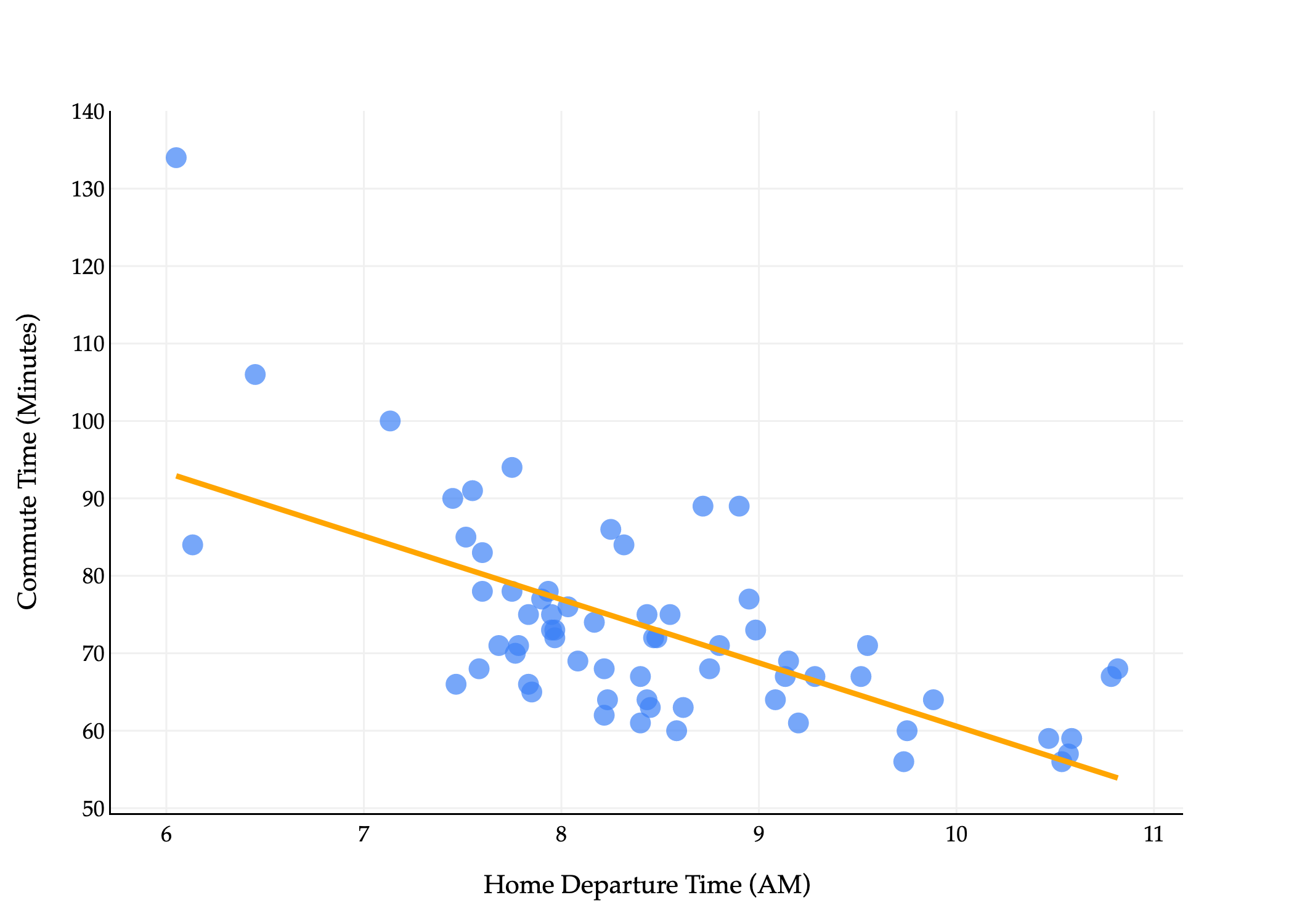
The line above goes by many names:
The simple linear regression line that minimizes mean squared error.
The simple linear regression line (if said without context).
The regression line.
The least squares regression line (because it has the least mean squared error).
The line of best fit.
Whatever you’d like to call it, now that we’ve found our optimal parameters, we can use them to make predictions.
On the dataset of commute times:
# Assume x is an array with departure hours and y is an array with commute times.
w1_star = np.sum((x - np.mean(x)) * (y - np.mean(y))) / np.sum((x - np.mean(x)) ** 2)
w0_star = np.mean(y) - w1_star * np.mean(x)

w0_star, w1_star
(142.4482415877287, -8.186941724265552)So, our specific fit, or trained hypothesis function is:
This trained hypothesis function is not saying that leaving later causes you to have shorter commutes. Rather, that’s just the best linear pattern it observed in the data for the purposes of minimizing mean squared error. In reality, there are other factors that affect commute times, and we haven’t performed a thorough-enough analysis to say anything about the causal relationship between departure time and commute time.
To predict how long it might take to get to school tomorrow, plug in the time you’d like to leave for and out will come your prediction. The slope, -8.19, is in units , and is telling us that for every hour later you leave, your predicted commute time decreases by 8.19 minutes.
In Python, I can define a predict function as follows:
def predict(x_new):
    return w0_star + w1_star * x_new

# Predicted commute time if I leave at 8:30AM.
predict(8.5)72.8592369314715Regression Line Passes Through the Mean
There’s an important property that the regression line satisfies: for any dataset, the line that minimizes mean squared error passes through the point .
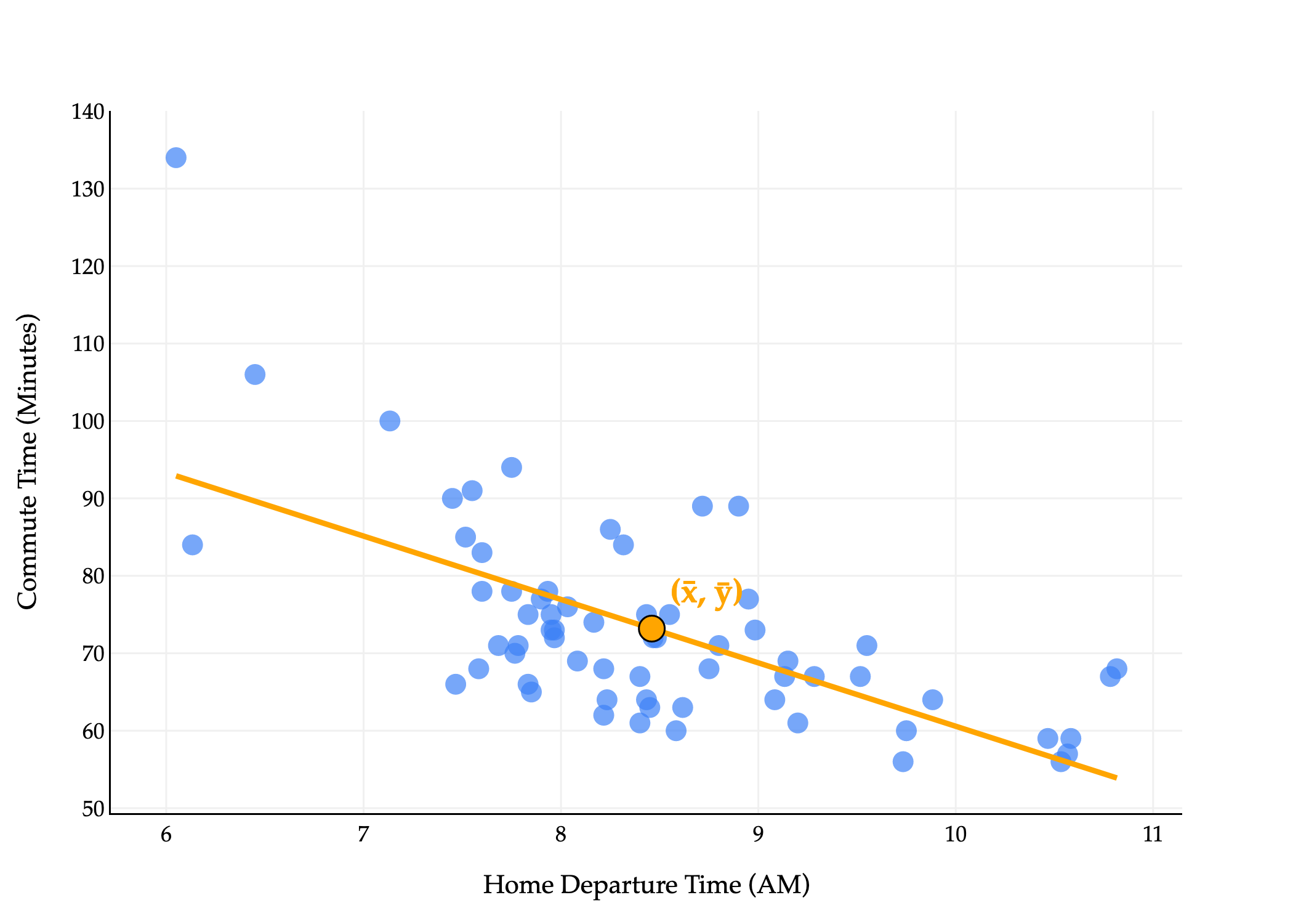
predict(np.mean(x))73.18461538461538# Same!
np.mean(y)73.18461538461538Our commute times regression line passes through the point , even if that was not necessarily one of the original points in the dataset.
Intuitively, this says that for an average input, the line that minimizes mean squared error will always predict an average output.
Why is this fact true? See if you can reason about it yourself, then check the solution once you’ve attempted it.
Proof that the regression line passes through
Our regression line is:
We know that the optimal intercept of the regression line is:
Substituting this in yields:
If we plug in , we have:
My interpretation of this is that the intercept is chosen to “vertically adjust” the line so that it passes through .
The Modeling Recipe
To conclude, let’s run through the three-step modeling recipe.
1. Choose a model.
2. Choose a loss function.
We chose squared loss:
3. Minimize average loss to find optimal parameters.
For the simple linear regression model, empirical risk is:
We showed that:
While the process of minimizing was much, much more complex than in the case of our single parameter model, the conceptual backing of the process was still this three-step recipe, and hopefully now you see its value.