6.5. The Gram-Schmidt Process - EECS 245 Course Notes

This section can be thought of as a detour through the main storyline of the course. Chapter 7.1 is where I connect the idea of projecting $\vec y$ onto the column space of $X$ to that of linear regression.

Instead, here I’ll introduce a new algorithm that can be used to turn a collection of vectors into a more convenient form, and see how this can make the act of projecting $\vec y$ onto the column space of $X$ much easier.

Why Orthogonalize?¶

Recall, a set of vectors $\vec q_1, \vec q_2, \ldots, \vec q_d \in \mathbb{R}^n$ are orthonormal if they are both:

pairwise orthogonal, meaning $\vec q_i \cdot \vec q_j = 0$ for all $i \neq j$ , and
each vector is a unit vector, meaning $\lVert \vec q_i \rVert = 1$ for all $i$

Orthonormal vectors (and matrices containing them) are convenient to work with. For example, if $Q$ ’s columns are the vectors $\vec q_1, \vec q_2, \ldots, \vec q_d$ , then $Q^TQ$ , the matrix containing the dot products of the columns of $Q$ , is the identity matrix.

Q^TQ = \begin{bmatrix} \vec q_1 \cdot \vec q_1 & \vec q_1 \cdot \vec q_2 & \cdots & \vec q_1 \cdot \vec q_d \\ \vec q_2 \cdot \vec q_1 & \vec q_2 \cdot \vec q_2 & \cdots & \vec q_2 \cdot \vec q_d \\ \vdots & \vdots & \ddots & \vdots \\ \vec q_d \cdot \vec q_1 & \vec q_d \cdot \vec q_2 & \cdots & \vec q_d \cdot \vec q_d \end{bmatrix} = \begin{bmatrix} 1 & 0 & \cdots & 0 \\ 0 & 1 & \cdots & 0 \\ \vdots & \vdots & \ddots & \vdots \\ 0 & 0 & \cdots & 1 \end{bmatrix} = I

(I know that I promised to use superscripts like $\vec q^{(1)}$ to denote columns of a matrix, but I have my reasons for doing it this way in this section.)

As we’ve seen in Chapter 6.3, when projecting $\vec y$ onto the column space of $X$ , the matrix $X^TX$ – and its inverse – plays a big role in finding the optimal coefficients $\vec w^*$ to multiply each column of $X$ by. Most matrices, by default, don’t have orthonormal columns. But if they did, then some of these calculations would be much, much simpler!

So, the goal here is to learn how to turn a linearly independent set of vectors into an orthonormal set of vectors with the same span, i.e. how to “orthogonalize” a set of vectors.

\underset{\text{linearly independent set of vectors}}{\vec v_1, \vec v_2, \ldots, \vec v_d} \to \underset{\text{orthonormal set of vectors with the same span}}{\vec q_1, \vec q_2, \ldots, \vec q_d}

The Algorithm¶

The algorithm that produces this orthonomal set of vectors is called the Gram-Schmidt process. It exploits the fact that when you project $\vec y$ onto $\vec x$ , the error vector

\vec e = \vec y - \vec p

is orthogonal to $\vec x$ .

# This chunk must be in the first plotting cell of each notebook in order to guarantee that the mathjax script is loaded.

import plotly
from IPython.display import display, HTML

plotly.offline.init_notebook_mode()
display(HTML(
    '<script type="text/javascript" async src="https://cdnjs.cloudflare.com/ajax/libs/mathjax/2.7.1/MathJax.js?config=TeX-MML-AM_SVG"></script>'
))

import numpy as np
import plotly.graph_objects as go

y = np.array([3, 1])
x = np.array([3, -2])

# Calculate k^* where error is orthogonal to x
k_star = np.dot(y, x) / np.dot(x, x)
p = k_star * x  # p = k^* x
e = y - p       # error vector (orthogonal to x)

def create_vector_trace(coords, color, label, opacity=1.0):
    x_coord, y_coord = coords
    return go.Scatter(
        x=[0, x_coord], 
        y=[0, y_coord],
        mode='lines+markers',
        line=dict(color=color, width=4),
        marker=dict(
            size=[0, 16],
            color=[color, color],
            symbol=['circle', 'arrow'],
            angleref='previous'
        ),
        hovertemplate='(%{x}, %{y})<extra></extra>',
        showlegend=False,
        name=label,
        opacity=opacity
    )

def create_error_trace(start_coords, end_coords, color, label, opacity=1.0):
    return go.Scatter(
        x=[start_coords[0], end_coords[0]], 
        y=[start_coords[1], end_coords[1]],
        mode='lines+markers',
        line=dict(color=color, width=3, dash='dot'),
        marker=dict(
            size=[0, 12],
            color=[color, color],
            symbol=['circle', 'arrow'],
            angleref='previous'
        ),
        hovertemplate='(%{x}, %{y})<extra></extra>',
        showlegend=False,
        name=label,
        opacity=opacity
    )

def plot_static_projection():
    traces = []

    traces.append(create_vector_trace(tuple(y), 'orange', r'$\vec y$'))
    traces.append(create_vector_trace(tuple(x), '#3d81f6', r'$\vec x$', opacity=0.5))
    traces.append(create_vector_trace(tuple(p), '#004d40', r'$\vec p = k^* \vec x$'))
    traces.append(create_error_trace(tuple(p), tuple(y), '#d81b60', r'$\vec e$'))

    x_unit = x / np.linalg.norm(x)
    e_unit = e / np.linalg.norm(e)
    marker_size = 0.12

    p0 = p
    p1 = p0 + -x_unit * marker_size
    p2 = p1 + e_unit * marker_size

    right_angle_trace = go.Scatter(
        x=[p1[0], p2[0], p2[0] - (p1[0] - p0[0])],
        y=[p1[1], p2[1], p2[1] - (p1[1] - p0[1])],
        mode='lines',
        line=dict(color="#222", width=2),
        showlegend=False,
        hoverinfo='skip'
    )
    traces.append(right_angle_trace)
    
    min_x_val = min(0, p[0], y[0], x[0]) - 0.5
    max_x_val = max(0, p[0], y[0], x[0]) + 1.5
    min_y_val = min(0, p[1], y[1], x[1]) - 0.5
    max_y_val = max(0, p[1], y[1], x[1]) + 1.5

    top_right_corner = (max_x_val - 0.2, max_y_val - 0.2)

    fig = go.Figure(data=traces)
    
    fig.add_annotation(
        x=y[0],
        y=y[1] + 0.13,
        text=r"$\vec y$",
        showarrow=False,
        font=dict(size=18, family="Palatino, serif", color="orange"),
        align="center"
    )
    fig.add_annotation(
        x=x[0] + 0.13,
        y=x[1] - 0.13,
        text=r"$\vec x$",
        showarrow=False,
        font=dict(size=18, family="Palatino, serif", color="#3d81f6"),
        align="center"
    )
    fig.add_annotation(
        x=p[0] - 1,
        y=p[1] + 0.2,
        text=fr"$\vec p = k^* \vec x$",
        showarrow=False,
        font=dict(size=18, family="Palatino, serif", color="#004d40"),
        align="left"
    )
    fig.add_annotation(
        x=p[0] - 1,
        y=p[1] + 0.2,
        text=fr"$\vec p = k^* \vec x$",
        showarrow=False,
        font=dict(size=18, family="Palatino, serif", color="#004d40"),
        align="left"
    )
    fig.add_annotation(
        x=(p[0] + y[0]) / 2 + 0.21,
        y=(p[1] + y[1]) / 2 + 0.03,
        text=r"$\vec e$",
        showarrow=False,
        font=dict(size=18, family="Palatino, serif", color="#d81b60"),
        align="center"
    )
    fig.update_layout(
        width=480,
        height=420,
        yaxis_scaleanchor="x",
        margin=dict(l=10, r=10, t=10, b=10),
        font=dict(family="Palatino, serif"),
        plot_bgcolor="white",
        paper_bgcolor="white",
    )
    fig.update_xaxes(
        range=[min_x_val, max_x_val],
        showticklabels=False,
        gridcolor="#fff",
        zerolinecolor="#fff"
    )
    fig.update_yaxes(
        range=[min_y_val, max_y_val],
        showticklabels=False,
        gridcolor="#fff",
        zerolinecolor="#fff"
    )
    return fig

plot_static_projection().show(renderer='png', scale=3)

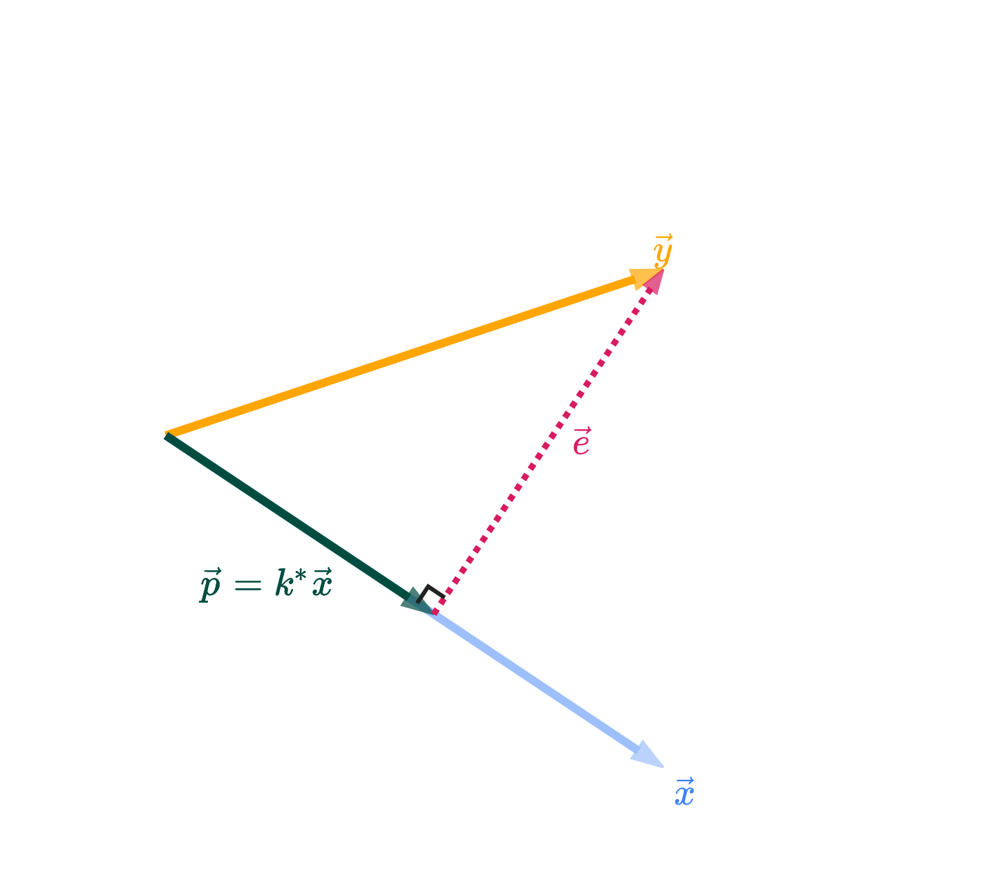
If you look in the figure above, the vectors $\color{#3d81f6} \vec x$ and $\color{#d81b60} \vec e$ are orthogonal, and have the same span as $\color{orange} \vec y$ and $\color{#3d81f6} \vec x$ . The key takeaway is that if you’d like to “invent” vectors that are orthogonal to each other, you can construct them by iteratively projecting!

To illustrate how the algorithm works, let’s use as an example the vectors

\vec v_1 = \begin{bmatrix} 1 \\ -1 \\ 1 \end{bmatrix}, \quad \vec v_2 = \begin{bmatrix} 1 \\ 0 \\ 1 \end{bmatrix}, \quad \vec v_3 = \begin{bmatrix} 1 \\ 1 \\ 2 \end{bmatrix}

These are three linearly independent vectors in $\mathbb{R}^3$ , though they are not orthogonal. These vectors span some subspace $S$ . Our goal is to find an orthonormal set of vectors that spans the same $S$ . (In this case, $S$ is all of $\mathbb{R}^3$ , but in general this process works even if $d < n$ .)

In what follows, let $\text{proj}_{\vec x}(\vec y)$ be the projection of $\vec y$ onto $\vec x$ , i.e. $\text{proj}_{\vec x}(\vec y) = \frac{\vec y \cdot \vec x}{\vec x \cdot \vec x} \vec x$ .

Iteration 1: Set ${\color{3d81f6} \vec Q_1} = \vec v_1$ .
In the first iteration, we simply take the first vector $\vec v_1$ and copy it to $\vec Q_1$ . From now on, each new vector will be constructed to be orthogonal to all previously constructed $\vec Q_i$ ’s.
$\color{3d81f6} \vec Q_1 = \begin{bmatrix} 1 \\ -1 \\ 1 \end{bmatrix}$
Iteration 2: Set ${\color{orange} \vec Q_2} = \vec v_2 - \text{proj}_{\color{3d81f6}\vec Q_1}(\vec v_2)$ .
$\color{orange} \vec Q_2$ is the same as the error vector from projecting $\vec v_2$ onto $\color{3d81f6} \vec Q_1$ , which we know is orthogonal to $\color{3d81f6} \vec Q_1$ .
Even without actually calculating $\color{orange} \vec Q_2$ , we can see that it, by definition, must be orthogonal to $\color{3d81f6} \vec Q_1$ .
$\begin{align*} {\color{orange} \vec Q_2} \cdot {\color{3d81f6} \vec Q_1} &= \left(\vec v_2 - \text{proj}_{\color{3d81f6}\vec Q_1}(\vec v_2)\right) \cdot {\color{3d81f6} \vec Q_1} \\ &= \left( \vec v_2- \frac{\vec v_2 \cdot {\color{3d81f6} \vec Q_1}}{{\color{3d81f6} \vec Q_1} \cdot {\color{3d81f6} \vec Q_1}} {\color{3d81f6} \vec Q_1} \right) \cdot {\color{3d81f6} \vec Q_1} \\ &= \vec v_2 \cdot {\color{3d81f6} \vec Q_1} - \frac{\vec v_2 \cdot {\color{3d81f6} \vec Q_1}}{{\color{3d81f6} \vec Q_1} \cdot {\color{3d81f6} \vec Q_1}} {\color{3d81f6} \vec Q_1} \cdot {\color{3d81f6} \vec Q_1} \\ &= \vec v_2 \cdot {\color{3d81f6} \vec Q_1} - \vec v_2 \cdot {\color{3d81f6} \vec Q_1} \\ &= 0 \end{align*}$
With that understanding in mind, let’s evaluate $\color{orange} \vec Q_2$ explicitly.
${\color{orange} \vec Q_2} = \underbrace{\begin{bmatrix} 1 \\ 0 \\ 1 \end{bmatrix}}_{\vec v_2} - \underbrace{\frac{\begin{bmatrix} 1 \\ 0 \\ 1 \end{bmatrix} \cdot \color{3d81f6} \begin{bmatrix} 1 \\ -1 \\ 1 \end{bmatrix}}{\color{3d81f6} \begin{bmatrix} 1 \\ -1 \\ 1 \end{bmatrix} \cdot \color{3d81f6} \begin{bmatrix} 1 \\ -1 \\ 1 \end{bmatrix}} \color{3d81f6} \begin{bmatrix} 1 \\ -1 \\ 1 \end{bmatrix}}_{\text{proj}_{\color{3d81f6}\vec Q_1}(\vec v_2)} = \begin{bmatrix} 1 \\ 0 \\ 1 \end{bmatrix} - \frac{2}{3} \color{3d81f6} \begin{bmatrix} 1 \\ -1 \\ 1 \end{bmatrix} = \color{orange} \begin{bmatrix} 1/3 \\ 2/3 \\ 1/3 \end{bmatrix}$
Iteration 3: Set ${\color{d81b60} \vec Q_3} = \vec v_3 - \text{proj}_{\color{3d81f6}\vec Q_1}(\vec v_3) - \text{proj}_{\color{orange}\vec Q_2}(\vec v_3)$ .
When constructed this way, $\color{d81b60} \vec Q_3$ is orthogonal to both $\color{3d81f6} \vec Q_1$ and $\color{orange} \vec Q_2$ . Think of it this way: $\text{span}(\{{\color{3d81f6} \vec Q_1}, {\color{orange} \vec Q_2}\})$ is a plane in $\mathbb{R}^3$ ; after projecting $\vec v_3$ onto this plane, the remaining part of $\vec v_3$ that is orthogonal to the plane is $\color{d81b60} \vec Q_3$ . If that doesn’t make sense, execute ${\color{d81b60} \vec Q_3} \cdot \color{3d81f6} \vec Q_1$ and ${\color{d81b60} \vec Q_3} \cdot \color{orange} \vec Q_2$ using the same general steps I followed in Iteration 2.

\begin{align*} {\color{d81b60} \vec Q_3} &= \vec v_3 - \text{proj}_{\color{3d81f6}\vec Q_1}(\vec v_3) - \text{proj}_{\color{orange}\vec Q_2}(\vec v_3) \\ &= \begin{bmatrix} 1 \\ 1 \\ 2 \end{bmatrix} - \underbrace{\frac{\begin{bmatrix} 1 \\ 1 \\ 2 \end{bmatrix} \cdot \color{3d81f6} \begin{bmatrix} 1 \\ -1 \\ 1 \end{bmatrix}}{\color{3d81f6} \begin{bmatrix} 1 \\ -1 \\ 1 \end{bmatrix} \cdot \color{3d81f6} \begin{bmatrix} 1 \\ -1 \\ 1 \end{bmatrix}} \color{3d81f6} \begin{bmatrix} 1 \\ -1 \\ 1 \end{bmatrix}}_{\text{proj}_{\color{3d81f6}\vec Q_1}(\vec v_3)} - \underbrace{\frac{\begin{bmatrix} 1 \\ 1 \\ 2 \end{bmatrix} \cdot \color{orange} \begin{bmatrix} 1/3 \\ 2/3 \\ 1/3 \end{bmatrix}}{\color{orange} \begin{bmatrix} 1/3 \\ 2/3 \\ 1/3 \end{bmatrix} \cdot \color{orange} \begin{bmatrix} 1/3 \\ 2/3 \\ 1/3 \end{bmatrix}} \color{orange} \begin{bmatrix} 1/3 \\ 2/3 \\ 1/3 \end{bmatrix}}_{\text{proj}_{\color{orange}\vec Q_2}(\vec v_3)} \\ &= \color{d81b60} \begin{bmatrix} -1/2 \\ 0 \\ 1/2 \end{bmatrix} \end{align*}

If there were more $\vec v_i$ ’s, we’d continue this process, each time constructing a new $\vec Q_i$ that is orthogonal to all previously constructed $\vec Q_i$ ’s by “subtracting off” the parts we’ve already accounted for through the earlier $\vec Q_i$ ’s.

Now, $\vec Q_1, \vec Q_2, \vec Q_3$ are orthogonal to one another, but they are not yet unit vectors. To make them unit vectors, we simply need to divide each by its length.

{\color{3d81f6} \vec q_1 = \frac{\color{3d81f6} \vec Q_1}{\lVert \color{3d81f6} \vec Q_1 \rVert} = \boxed{\begin{bmatrix} 1 /\sqrt{3} \\ -1 /\sqrt{3} \\ 1 /\sqrt{3} \end{bmatrix}}} \\ {\color{orange} \vec q_2 = \frac{\color{orange} \vec Q_2}{\lVert \color{orange} \vec Q_2 \rVert} = \boxed{\begin{bmatrix} 1 /\sqrt{6} \\ 2 /\sqrt{6} \\ 1 /\sqrt{6} \end{bmatrix}}} \\ \color{d81b60} \vec q_3 = \frac{\color{d81b60} \vec Q_3}{\lVert \color{d81b60} \vec Q_3 \rVert} = \boxed{\begin{bmatrix} -1 /\sqrt{2} \\ 0 \\ 1 /\sqrt{2} \end{bmatrix}}

Now, the vectors $\vec q_1, \vec q_2, \vec q_3$ are orthonormal to one another, and they span the same subspace $S$ as the vectors $\vec v_1, \vec v_2, \vec v_3$ !

A quick note on signs: you could multiply any of the $\vec q_i$ ’s by -1 without changing the span of the collection, so if using a computer to compute the $\vec q_i$ ’s, you might see them come out with different signs.

import numpy as np
from plotly.subplots import make_subplots

from utils import plot_vectors

v1 = np.array([1, -1, 1])
v2 = np.array([1, 0, 1])
v3 = np.array([1, 1, 2])

q1 = np.array([1 / np.sqrt(3), -1 / np.sqrt(3), 1 / np.sqrt(3)])
q2 = np.array([1 / np.sqrt(6), 2 / np.sqrt(6), 1 / np.sqrt(6)])
q3 = np.array([-1 / np.sqrt(2), 0, 1 / np.sqrt(2)])

before = [
    (tuple(v1), '#3d81f6', 'v₁'),
    (tuple(v2), 'orange', 'v₂'),
    (tuple(v3), '#d81b60', 'v₃')
]

after = [
    (tuple(q1), '#3d81f6', 'q₁'),
    (tuple(q2), 'orange', 'q₂'),
    (tuple(q3), '#d81b60', 'q₃')
]

# Show axis labels on the bottom (orthonormal) plot, but hide on the top for clarity
left_fig = plot_vectors(before, show_axis_labels=False)
right_fig = plot_vectors(after, show_axis_labels=False)

fig = make_subplots(
    rows=2,
    cols=1,
    specs=[[{'type': 'scene'}], [{'type': 'scene'}]],
    subplot_titles=('Before Gram-Schmidt', 'After Gram-Schmidt'),
    vertical_spacing=0.05
)

for trace in left_fig.data:
    fig.add_trace(trace, row=1, col=1)

for trace in right_fig.data:
    fig.add_trace(trace, row=2, col=1)

axis_range = [-2.5, 2.5]

shared_axis_top = dict(
    dtick=1, range=axis_range,
    showbackground=True, backgroundcolor='white',
    gridcolor='#f0f0f0', showticklabels=False,
    title=None, zerolinecolor='gray'
)

top_scene_style = dict(
    xaxis=shared_axis_top,
    yaxis=shared_axis_top,
    zaxis=shared_axis_top,
    camera=dict(eye=dict(x=0.95, y=1.3, z=0.4)),
    aspectmode='cube',
    bgcolor='white'
)

def labeled_axis(title):
    return dict(
        dtick=1, range=axis_range,
        showbackground=True, backgroundcolor='white',
        gridcolor='#f0f0f0', showticklabels=True,
        title=title, zerolinecolor='gray'
    )

bottom_scene_style = dict(
    xaxis=labeled_axis('x'),
    yaxis=labeled_axis('y'),
    zaxis=labeled_axis('z'),
    camera=dict(eye=dict(x=0.95, y=1.3, z=0.4)),
    aspectmode='cube',
    bgcolor='white'
)

fig.update_layout(
    scene=top_scene_style,
    scene2=bottom_scene_style,
    width=800,
    height=900,
    paper_bgcolor='white',
    plot_bgcolor='white',
    font=dict(family='Palatino', size=16),
    margin=dict(l=10, r=10, t=50, b=10)
)

fig.show()

Notice above that $\color{3d81f6} \vec v_1$ in the top and $\color{3d81f6} \vec q_1$ in the bottom are parallel, it’s just that $\color{3d81f6} \vec q_1$ is a unit vector. The three $\vec v_i$ ’s in the top figure are linearly independent but not orthogonal; the three $\vec q_i$ ’s in the bottom figure are, however, orthonormal.

Gram-Schmidt and Projection¶

In general, we’re presumed to have a vector $\vec y$ that we’d like to approximate as a linear combination of matrix $X$ ’s columns. Generally, $X$ ’s columns are not orthonormal – they may not even be linearly independent.

If we:

Remove the linearly dependent columns from $X$
Use the Gram-Schmidt process to orthonormalize the remaining columns, and store them in the columns of $Q$

Then, the matrix $Q$ that results has the same column space as $X$ , but solving the normal equations for $Q$ and $\vec y$ is much simpler.

Our problem now is slightly different: we’re trying to find the best linear combination of the columns of $Q$ (not the columns of $X$ ) that approximates $\vec y$ , i.e. we’re projecting $\vec y$ onto the column space of $Q$ . If we adjust our objective to this goal, then the best $\vec w^*$ – the one that minimizes $\lVert \vec y - Q \vec w \rVert^2$ – satisfies

Q^TQ \vec w = Q^T \vec y

But, $Q^TQ = I$ as I showed you at the start of this section, so this just reduces to

\vec w^* = Q^T \vec y

That’s it! No inversion required: we can compute $\vec w^*$ with just a single matrix-vector multiplication.