Chapter 6: Linear Transformations and Projections

Sections¶

• 6.1. Linear Transformations
• 6.2. Inverses
• 6.3. Projecting onto the Column Space
• 6.4. The Complete Solution to the Normal Equations
• 6.5. The Gram-Schmidt Process

Summary¶

6.1 Linear Transformations¶

• A function $T: \mathbb{R}^d \to \mathbb{R}^n$ is a linear transformation if it satisfies both properties:

  $$T(\vec x + \vec y) = T(\vec x) + T(\vec y)$$
  $$T(c\vec x) = cT(\vec x)$$

• Matrix representation: every linear transformation has the form

  $$T(\vec x) = A\vec x$$

• Linear transformations send $\vec 0$ to $\vec 0$.

• $A\vec x + \vec b$ is affine; it is not linear when $\vec b \ne \vec 0$.

• A $2 \times 2$ matrix maps the unit square to the parallelogram created by its columns. For example,

  $$A = \begin{bmatrix} 2 & 1 \\ 1 & 2 \end{bmatrix}$$
  

• Composition: $AB\vec x$ applies $B$ first, then $A$.

• Counterclockwise rotation by $\theta$:

  $$R(\theta) = \begin{bmatrix} \cos\theta & -\sin\theta \\ \sin\theta & \cos\theta \end{bmatrix}$$

• Determinant of a $2 \times 2$ matrix:

  $$\det\left(\begin{bmatrix} a & b \\ c & d \end{bmatrix}\right) = \begin{vmatrix} a & b \\ c & d \end{vmatrix} = ad - bc$$

• Determinant of a $3 \times 3$ matrix:

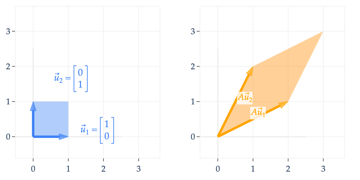
  $$\det\left(\begin{bmatrix} {\color{#3d81f6} a} & {\color{#3d81f6} b} & {\color{#3d81f6} c} \\ {\color{orange} d} & {\color{#d81a60}e } & {\color{#004d40}f } \\ {\color{orange} g} & {\color{#d81a60}h } & {\color{#004d40}i } \end{bmatrix}\right) = \begin{vmatrix} {\color{#3d81f6} a} & {\color{#3d81f6} b} & {\color{#3d81f6} c} \\ {\color{orange} d} & {\color{#d81a60}e } & {\color{#004d40}f } \\ {\color{orange} g} & {\color{#d81a60}h } & {\color{#004d40}i } \end{vmatrix}$$
  $$\begin{vmatrix} {\color{#3d81f6} a} & {\color{#3d81f6} b} & {\color{#3d81f6} c} \\ {\color{orange} d} & {\color{#d81a60}e } & {\color{#004d40}f } \\ {\color{orange} g} & {\color{#d81a60}h } & {\color{#004d40}i } \end{vmatrix} = {\color{#3d81f6} a} \begin{vmatrix} {\color{#d81a60}e } & {\color{#004d40}f } \\ {\color{#d81a60}h } & {\color{#004d40}i } \end{vmatrix} - {\color{#3d81f6} b} \begin{vmatrix} {\color{orange} d} & {\color{#004d40}f } \\ {\color{orange} g} & {\color{#004d40}i } \end{vmatrix} + {\color{#3d81f6} c} \begin{vmatrix} {\color{orange} d} & {\color{#d81a60}e } \\ {\color{orange} g} & {\color{#d81a60}h } \end{vmatrix}$$

• Geometric interpretation: $\det(A)$ is the signed area (volume) that the unit square (cube) maps to.

• $\det(A) = 0$ iff the columns of $A$ are dependent.

• Determinant of a transpose:

  $$\det(A^T) = \det(A)$$

• Determinant of a product:

  $$\det(AB) = \det(A)\det(B)$$

• Scaling an $n \times n$ matrix:

  $$\det(cA) = c^n\det(A)$$

• Swapping two columns or two rows flips the sign of the determinant.

• An orthogonal matrix $Q$ has $\det(Q) = \pm 1$.

6.2 Inverses¶

• Inverse: for a square matrix $A$, its inverse satisfies

  $$AA^{-1} = A^{-1}A = I$$

• For an $n \times n$ matrix $A$, the following are equivalent:

  • $A$ is invertible.

  • $\text{rank}(A) = n$.

  • The columns (and rows) of $A$ are linearly independent.

  • $\text{nullsp}(A) = \{\vec 0\}$.

  • $\det(A) \ne 0$.

  • $A\vec x = \vec b$ has exactly one solution for every $\vec b \in \mathbb{R}^n$.

• Inverse of a $2 \times 2$ matrix, when $ad - bc \ne 0$:

  $$\begin{bmatrix} a & b \\ c & d \end{bmatrix}^{-1} = \frac{1}{ad - bc}\begin{bmatrix} d & -b \\ -c & a \end{bmatrix}$$

• Inverse of a product: the order reverses.

  $$(AB)^{-1} = B^{-1}A^{-1}$$

• Inverse of a transpose:

  $$(A^T)^{-1} = (A^{-1})^T$$

• Inverse of an orthogonal matrix: since $Q^TQ = QQ^T = I$,

  $$Q^{-1} = Q^T$$

• Because $\text{rank}(X^TX) = \text{rank}(X)$, for the $d \times d$ matrix $X^TX$ to be invertible we need $\text{rank}(X^TX) = d$, meaning $\text{rank}(X) = d$, meaning all $d$ of $X$’s columns are linearly independent.

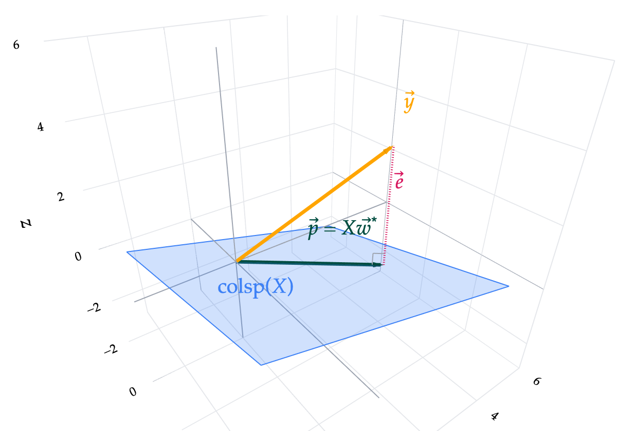
6.3 Projecting onto the Column Space¶

• For $X \in \mathbb{R}^{n \times d}$ and $\vec y \in \mathbb{R}^n$, the $\vec w$ that minimizes $\lVert \vec y - X\vec w \rVert^2$ makes the error vector orthogonal to $\text{colsp}(X)$.

  

• Error vector:

  $$\vec e = \vec y - X\vec w^*$$

• Orthogonality condition:

  $$X^T\vec e = \vec 0$$

• Normal equations: a system of $d$ equations in $d$ unknowns (the entries of $\vec w^*$).

  $$X^TX\vec w^* = X^T\vec y$$

• Unique solution, when $\text{rank}(X) = d$:

  $$\vec w^* = (X^TX)^{-1}X^T\vec y$$

• Projection of $\vec y$ onto $\text{colsp}(X)$:

  $$\vec p = X\vec w^*$$

• The error vector belongs to $\text{nullsp}(X^T)$.

• If $\vec 1 \in \text{colsp}(X)$, the errors sum to 0.

6.4 The Complete Solution to the Normal Equations¶

• The normal equations always have at least one solution; they may have exactly one solution or infinitely many.

• Complete solution: when $X$ has linearly dependent columns, there are infinitely many solutions to $X^TX\vec w^* = X^T\vec y$, all with the same $\vec p$:

  $$\vec w = \vec w_s + \vec n, \qquad \vec n \in \text{nullsp}(X)$$

• To find one solution $\vec w_s$, solve without the dependent columns, then put 0 in their slots.

• Projection matrix:

  • With linearly independent columns, the $n \times n$ matrix is

    $$P = X(X^TX)^{-1}X^T$$

  • Applying the projection matrix:

    $$\vec p = P\vec y$$

  • Symmetry: $P^T = P$.

  • Idempotence: $P^2 = P$.

  • Projection preserves the columns of $X$: $PX = X$.

  • Rank: $\text{rank}(P) = \text{rank}(X)$.

  • A projection matrix is invertible only when $P = I$.

• Rotation matrices are orthogonal and have determinant 1.

• Reflection across the hyperplane normal to a unit vector $\vec u$: the matrix is orthogonal and has determinant -1.

  $$I - 2\vec u\vec u^T$$

6.5 The Gram-Schmidt Process¶

• Gram-Schmidt turns linearly independent vectors into orthonormal vectors with the same span.

• Remove projections onto the previously constructed vectors:

  $$\vec Q_i = \vec v_i - \sum_{j=1}^{i-1} \frac{\vec v_i \cdot \vec Q_j}{\vec Q_j \cdot \vec Q_j}\,\vec Q_j$$

  Project onto the new $\vec Q_j$’s.

• Normalize:

  $$\vec q_i = \frac{\vec Q_i}{\lVert \vec Q_i \rVert}$$

• With the $\vec q_i$’s as columns, $Q$ has orthonormal columns: $Q^TQ = I$.

• If $X$ has orthonormal columns, the normal equations $X^TX\vec w^* = X^T\vec y$ reduce to

  $$\vec w^* = X^T\vec y$$