Suppose u and v are any two vectors in Rn. (When I say this, I just mean that they both have the same number of components.)
Let’s think about all possible vectors of the form kv, where k can be any scalar. Any vector of the form kv is a scalar multiple of v, and points in the same direction as v (if k>0) or the opposite direction (if k<0). What is different about these scalar multiples is how long they are.
To get a sense of what I mean by this, play with the slider for k below. There are three vectors being visualized: some u, some v, and kv, which depends on the value of k you choose.
# This chunk must be in the first plotting cell of each notebook in order to guarantee that the mathjax script is loaded.

import plotly
from IPython.display import display, HTML

plotly.offline.init_notebook_mode()
display(HTML(
    '<script type="text/javascript" async src="https://cdnjs.cloudflare.com/ajax/libs/mathjax/2.7.1/MathJax.js?config=TeX-MML-AM_SVG"></script>'
))

import numpy as np
import plotly.graph_objects as go

u = np.array([3, 1])
v = np.array([3, -2])

def create_vector_trace(coordinates, color, label):
    x, y = coordinates
    return go.Scatter(
        x=[0, x],
        y=[0, y],
        mode='lines+markers',
        line=dict(color=color, width=4),
        marker=dict(
            size=[0, 16],
            color=[color, color],
            symbol=['circle', 'arrow'],
            angleref='previous'
        ),
        hovertemplate='(%{x}, %{y})<extra></extra>',
        showlegend=False,
        name=label
    )

def make_traces(k, show_error):
    traces = []
    traces.append(create_vector_trace(tuple(u), 'orange', r'$\vec u$'))
    traces.append(create_vector_trace(tuple(v), 'rgba(61,129,246,0.5)', r'$\vec v$'))
    kv = k * v
    traces.append(create_vector_trace(tuple(kv), '#004d40', r'$k\vec v$'))
    error = u - kv
    if show_error:
        traces.append(go.Scatter(
            x=[kv[0], u[0]],
            y=[kv[1], u[1]],
            mode='lines+markers',
            line=dict(color='#d81b60', width=3, dash='dot'),
            marker=dict(
                size=[0, 12],
                color=['#d81b60', '#d81b60'],
                symbol=['circle', 'arrow'],
                angleref='previous'
            ),
            hovertemplate='(%{x}, %{y})<extra></extra>',
            showlegend=False,
            name=fr'$\vec u - {k:.2f}\vec v$'
        ))
    return traces, kv, error

def plot_projection(title, show_error):
    k_vals = np.linspace(-1, 2.0, 101)
    k0 = 0.83
    traces, kv, error = make_traces(k0, show_error)
    fig = go.Figure(data=traces)

    # Permanent annotations for u and v
    fig.add_annotation(
        x=0.5 * u[0],
        y=0.5 * u[1] + 0.5,
        text=r"$\vec u$",
        showarrow=False,
        font=dict(size=14, family="Palatino, serif", color="orange"),
        align="center"
    )
    fig.add_annotation(
        x=0.5 * v[0],
        y=0.5 * v[1] - 0.6,
        text=r"$\vec v$",
        showarrow=False,
        font=dict(size=14, family="Palatino, serif", color="#3d81f6"),
        align="center"
    )
    # k annotation
    fig.add_annotation(
        x=kv[0] + 0.5,
        y=kv[1] - 1,
        text=fr"$k \vec v = {k0:.2f} \vec v$",
        showarrow=False,
        font=dict(size=14, family="Palatino, serif", color="#004d40"),
        align="center"
    )
    # error annotation (only if show_error)
    if show_error:
        fig.add_annotation(
            x=kv[0] + 0.5 * (u[0] - kv[0]) + 1,
            y=kv[1] + 0.5 * (u[1] - kv[1]) - 0.5,
            text=fr"$\vec e = \vec u - ({k0:.2f}\vec v)$",
            showarrow=False,
            font=dict(size=14, family="Palatino, serif", color="#d81b60"),
            align="center"
        )

    # Frames for animation/slider
    frames = []
    for k in k_vals:
        traces, kv, error = make_traces(k, show_error)
        annots = [
            dict(
                x=0.5 * u[0],
                y=0.5 * u[1] + 0.5,
                text=r"$\vec u$",
                showarrow=False,
                font=dict(size=14, family="Palatino, serif", color="orange"),
                align="center"
            ),
            dict(
                x=0.5 * v[0],
                y=0.5 * v[1] - 0.6,
                text=r"$\vec v$",
                showarrow=False,
                font=dict(size=14, family="Palatino, serif", color="#3d81f6"),
                align="center"
            ),
            dict(
                x=kv[0] + 0.5,
                y=kv[1] - 1,
                text=fr"$k \vec v = {k:.2f} \vec v$",
                showarrow=False,
                font=dict(size=14, family="Palatino, serif", color="#004d40"),
                align="center"
            )
        ]
        if show_error:
            annots.append(
                dict(
                    x=kv[0] + 0.5 * (u[0] - kv[0]) + 1,
                    y=kv[1] + 0.5 * (u[1] - kv[1]) - 0.5,
                    text=fr"$\vec e = \vec u - ({k:.2f}\vec v)$",
                    showarrow=False,
                    font=dict(size=14, family="Palatino, serif", color="#d81b60"),
                    align="center"
                )
            )
        frames.append(go.Frame(
            data=traces,
            name=f"{k:.2f}",
            layout=go.Layout(
                annotations=annots
            )
        ))
    fig.frames = frames

    # Slider steps
    steps = []
    for i, k in enumerate(k_vals):
        step = dict(
            method="animate",
            args=[
                [f"{k:.2f}"],
                {"mode": "immediate", "frame": {"duration": 0, "redraw": True}, "transition": {"duration": 0}}
            ],
            label=f"{k:.2f}"
        )
        steps.append(step)

    sliders = [dict(
        active=int((k0 - k_vals[0]) / (k_vals[1] - k_vals[0])),
        currentvalue={"prefix": "k = "},
        pad={"t": 30},
        steps=steps,
        minorticklen=0
    )]

    fig.update_layout(
        title=title,
        width=600,
        height=500,
        yaxis_scaleanchor="x",
        margin=dict(l=10, r=10, t=30, b=10),
        sliders=sliders,
        font=dict(family="Palatino, serif"),
        plot_bgcolor="white",
        paper_bgcolor="white",
        xaxis=dict(
            gridcolor="#f0f0f0",
            zerolinecolor="#f0f0f0"
        ),
        yaxis=dict(
            gridcolor="#f0f0f0",
            zerolinecolor="#f0f0f0"
        ),
    )
    fig.update_xaxes(range=[-3, 6], tickvals=np.arange(-4, 10), gridcolor="#f0f0f0", zerolinecolor="#f0f0f0")
    fig.update_yaxes(range=[-4, 2], tickvals=np.arange(-4, 4), gridcolor="#f0f0f0", zerolinecolor="#f0f0f0")
    fig.show(renderer="notebook")

plot_projection("", False)
Loading...
Loading...
Loading...
Loading...
Notice that the set of vectors of the form kv fill out a line. So really, what we’re asking is which vector on this line is closest to u.
In terms of angles, if θ is the angle between u and v, then the angle between u and kv is either θ (if k>0) or 180∘−θ (if k<0). So changing k doesn’t change how “similar” u and kv are in the cosine similarity sense.
But, some choices of k will make kv closer to u than others. I call this the approximation problem: how well can we recreate, or approximate, u using a scalar multiple of v? It turns out that linear regression is intimately related to this problem. Previously, we were trying to approximate commute times as best as we could using a linear function of departure times.
Let’s be more precise by what we mean by “closer”. For any value of k, we can measure the error of our approximation by the length of the error vector, e=u−kv.
plot_projection("", True)
Loading...
Loading...
Continue to play with the slider above for k. How do you get the length of the error vector to be as small as possible?
Intuitively, it seems that to get the error vectore to be as short as possible, we should make it orthogonal to v. Since we can control k, we can control u−kv, so we can make the error vector orthogonal to v by choosing the right k.
Our goal is to minimize the length of the error vector ∥e∥.
∥e∥
This is the same as minimizing
∥u−kv∥
One way to approach this problem is to treat the above expression as a function of k and find the value of k that minimizes it through calculus. You’ll do this in Homework 3. I’ll show you a more geometric approach here.
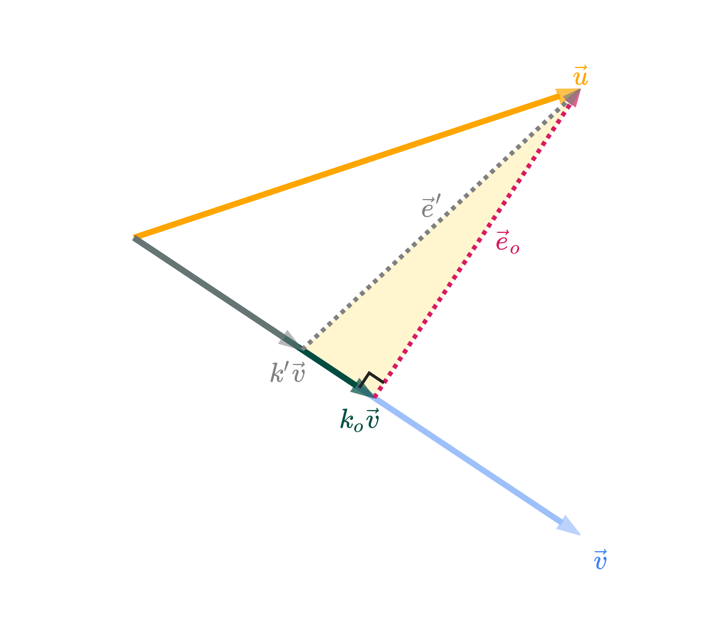
We’ve guessed, but not yet shown that the shortest possible error vector is the one that is orthogonal to v. Let ko be the value of k that makes the error vector eo=u−kovorthogonal to v. Here, we’ll prove that ko is the “best” choice of k by showing that any other choice of k will result in an error vector that is longer than eo. Think of this as a proof by contradiction (if you’re familiar with that idea; no worries if not).
For comparison, let k′ be some other value of k, and let its error vector be e′=u−k′v.
# This chunk must be in the first plotting cell of each notebook in order to guarantee that the mathjax script is loaded.

import plotly
from IPython.display import display, HTML

plotly.offline.init_notebook_mode()
display(HTML(
    '<script type="text/javascript" async src="https://cdnjs.cloudflare.com/ajax/libs/mathjax/2.7.1/MathJax.js?config=TeX-MML-AM_SVG"></script>'
))

import numpy as np
import plotly.graph_objects as go

u = np.array([3, 1])
v = np.array([3, -2])

# Calculate k_o where error is orthogonal to v
k_o = np.dot(u, v) / np.dot(v, v)
k_prime = k_o * 0.7  # Make k' slightly shorter than k_o

def create_vector_trace(coordinates, color, label, opacity=1.0):
    x, y = coordinates
    return go.Scatter(
        x=[0, x],
        y=[0, y],
        mode='lines+markers',
        line=dict(color=color, width=4),
        marker=dict(
            size=[0, 16],
            color=[color, color],
            symbol=['circle', 'arrow'],
            angleref='previous'
        ),
        hovertemplate='(%{x}, %{y})<extra></extra>',
        showlegend=False,
        name=label,
        opacity=opacity
    )

def create_error_trace(start_coords, end_coords, color, label, opacity=1.0):
    return go.Scatter(
        x=[start_coords[0], end_coords[0]],
        y=[start_coords[1], end_coords[1]],
        mode='lines+markers',
        line=dict(color=color, width=3, dash='dot'),
        marker=dict(
            size=[0, 12],
            color=[color, color],
            symbol=['circle', 'arrow'],
            angleref='previous'
        ),
        hovertemplate='(%{x}, %{y})<extra></extra>',
        showlegend=False,
        name=label,
        opacity=opacity
    )

def plot_static_projection():
    # Calculate vectors
    k_o_v = k_o * v
    k_prime_v = k_prime * v
    e_o = u - k_o_v  # Error vector for k_o (orthogonal to v)
    e_prime = u - k_prime_v  # Error vector for k_prime

    # Create traces
    traces = []

    # --- SHADE THE RIGHT-ANGLED TRIANGLE ---
    # The triangle vertices are: k_prime_v, k_o_v, u
    triangle_x = [k_prime_v[0], k_o_v[0], u[0], k_prime_v[0]]
    triangle_y = [k_prime_v[1], k_o_v[1], u[1], k_prime_v[1]]
    triangle_trace = go.Scatter(
        x=triangle_x,
        y=triangle_y,
        fill='toself',
        fillcolor='rgba(255, 215, 64, 0.25)',  # light gold, semi-transparent
        line=dict(color='rgba(255, 215, 64, 0.0)', width=0),  # no border
        mode='lines',
        showlegend=False,
        hoverinfo='skip'
    )
    traces.append(triangle_trace)
    # --- END SHADE ---

    # Original vectors u and v
    traces.append(create_vector_trace(tuple(u), 'orange', r'$\vec u$'))
    traces.append(create_vector_trace(tuple(v), '#3d81f6', r'$\vec v$', opacity=0.5))

    # k_o * v (optimal projection) - now #004d40
    traces.append(create_vector_trace(tuple(k_o_v), '#004d40', r'$k_o \vec v$'))

    # k' * v (shorter projection) - now gray
    traces.append(create_vector_trace(tuple(k_prime_v), 'gray', r"$k' \vec v$", opacity=0.8))

    # Error vector e_o (orthogonal to v)
    traces.append(create_error_trace(tuple(k_o_v), tuple(u), '#d81b60', r'$\vec e_o$'))

    # Error vector e' (for k') - now gray
    traces.append(create_error_trace(tuple(k_prime_v), tuple(u), 'gray', r"$\vec e'$"))

    # Add right angle symbol at the base of e_o
    # We'll draw a small right angle marker at the base (k_o_v) between v and e_o
    # The right angle marker will be a small "L" shape

    # Compute unit vectors for v and e_o
    v_unit = v / np.linalg.norm(v)
    e_o_unit = e_o / np.linalg.norm(e_o)
    # The right angle marker will be offset a small distance from k_o_v along v_unit and e_o_unit
    marker_size = 0.12  # controls the size of the right angle symbol

    # Start at k_o_v, move a bit along v_unit, then a bit along e_o_unit to form the "L"
    p0 = k_o_v
    p1 = p0 + -v_unit * marker_size
    p2 = p1 + e_o_unit * marker_size

    right_angle_trace = go.Scatter(
        x=[p1[0], p2[0], p2[0] - (p1[0] - p0[0])],
        y=[p1[1], p2[1], p2[1] - (p1[1] - p0[1])],
        mode='lines',
        line=dict(color="#222", width=2),
        showlegend=False,
        hoverinfo='skip'
    )
    traces.append(right_angle_trace)

    fig = go.Figure(data=traces)

    # Add annotations, positioned tightly to the relevant vectors/points
    # u vector (at tip)
    fig.add_annotation(
        x=u[0],
        y=u[1] + 0.13,
        text=r"$\vec u$",
        showarrow=False,
        font=dict(size=18, family="Palatino, serif", color="orange"),
        align="center"
    )

    # v vector (at tip)
    fig.add_annotation(
        x=v[0] + 0.13,
        y=v[1] - 0.13,
        text=r"$\vec v$",
        showarrow=False,
        font=dict(size=18, family="Palatino, serif", color="#3d81f6"),
        align="center"
    )

    # k_o * v (at tip) - now #004d40
    fig.add_annotation(
        x=k_o_v[0] + -0.1,
        y=k_o_v[1] - 0.13,
        text=fr"$k_o \vec v$",
        showarrow=False,
        font=dict(size=18, family="Palatino, serif", color="#004d40"),
        align="left"
    )

    # k' * v (at tip) - now gray
    fig.add_annotation(
        x=k_prime_v[0] - 0.1,
        y=k_prime_v[1] - 0.13,
        text=fr"$k' \vec v$",
        showarrow=False,
        font=dict(size=18, family="Palatino, serif", color="gray"),
        align="right"
    )

    # e_o error vector (midpoint between k_o*v and u, offset slightly)
    fig.add_annotation(
        x=(k_o_v[0] + u[0]) / 2 + 0.21,
        y=(k_o_v[1] + u[1]) / 2 + 0.03,
        text=r"$\vec e_o$",
        showarrow=False,
        font=dict(size=18, family="Palatino, serif", color="#d81b60"),
        align="center"
    )

    # e' error vector (midpoint between k'*v and u, offset slightly) - now gray
    fig.add_annotation(
        x=(k_prime_v[0] + u[0]) / 2 - 0.08,
        y=(k_prime_v[1] + u[1]) / 2 + 0.12,
        text=r"$\vec e'$",
        showarrow=False,
        font=dict(size=18, family="Palatino, serif", color="gray"),
        align="center"
    )

    # Triangle side annotation (midpoint between k_o*v and k'*v, offset slightly)
    # fig.add_annotation(
    #     x=(k_prime_v[0] + k_o_v[0]) / 2 - 0.08,
    #     y=(k_prime_v[1] + k_o_v[1]) / 2 - 0.13,
    #     text=r"$(k_o - k') \vec v$",
    #     showarrow=False,
    #     font=dict(size=15, family="Palatino, serif", color="purple"),
    #     align="center"
    # )

    # Update layout: tightly clip axes around the figure
    min_x = min(0, k_prime_v[0], k_o_v[0], u[0], v[0]) - 0.5
    max_x = max(0, k_prime_v[0], k_o_v[0], u[0], v[0]) + 0.5
    min_y = min(0, k_prime_v[1], k_o_v[1], u[1], v[1]) - 0.5
    max_y = max(0, k_prime_v[1], k_o_v[1], u[1], v[1]) + 0.5

    fig.update_layout(
        width=480,
        height=420,
        yaxis_scaleanchor="x",
        margin=dict(l=10, r=10, t=10, b=10),
        font=dict(family="Palatino, serif"),
        plot_bgcolor="white",
        paper_bgcolor="white",
    )
    fig.update_xaxes(
        range=[min_x, max_x],
        showticklabels=False,
        gridcolor="#fff",
        zerolinecolor="#fff"
    )
    fig.update_yaxes(
        range=[min_y, max_y],
        showticklabels=False,
        gridcolor="#fff",
        zerolinecolor="#fff"
    )

    # Show as static PNG
    return fig

plot_static_projection().show(renderer='png', scale=3)
Loading...
Loading...
I’ve drawn k′v in gray. Arbitrarily, I’ve shown it as being shorter than kov, but I could have drawn it as being longer and the argument would be the same. The prime has nothing to do with derivatives, by the way – it’s just a new variable.
The vectors k′v and kov, along with their corresponding error vectors, create a right-angled triangle, shaded in gold above. This triangle has a hypotenuse of e′ and legs of eo and k′v−kov.
Applying the Pythagorean theorem to this triangle gives us
∥e′∥2=∥eo∥2+>0∥k′v−kov∥2
∥k′v−kov∥2≥0, with equality only when we choose k′=ko, but we’ve assumed that k′=ko.
This implies that
∥e′∥2=∥eo∥2+some positive number
which means that ∥e′∥2>∥eo∥2.
In other words, if k′=ko, then ∥e′∥>∥eo∥. Thus, the error vector eo is shorter than any other error vector e′, and the best choice of k is ko!
What was the point of all this again?
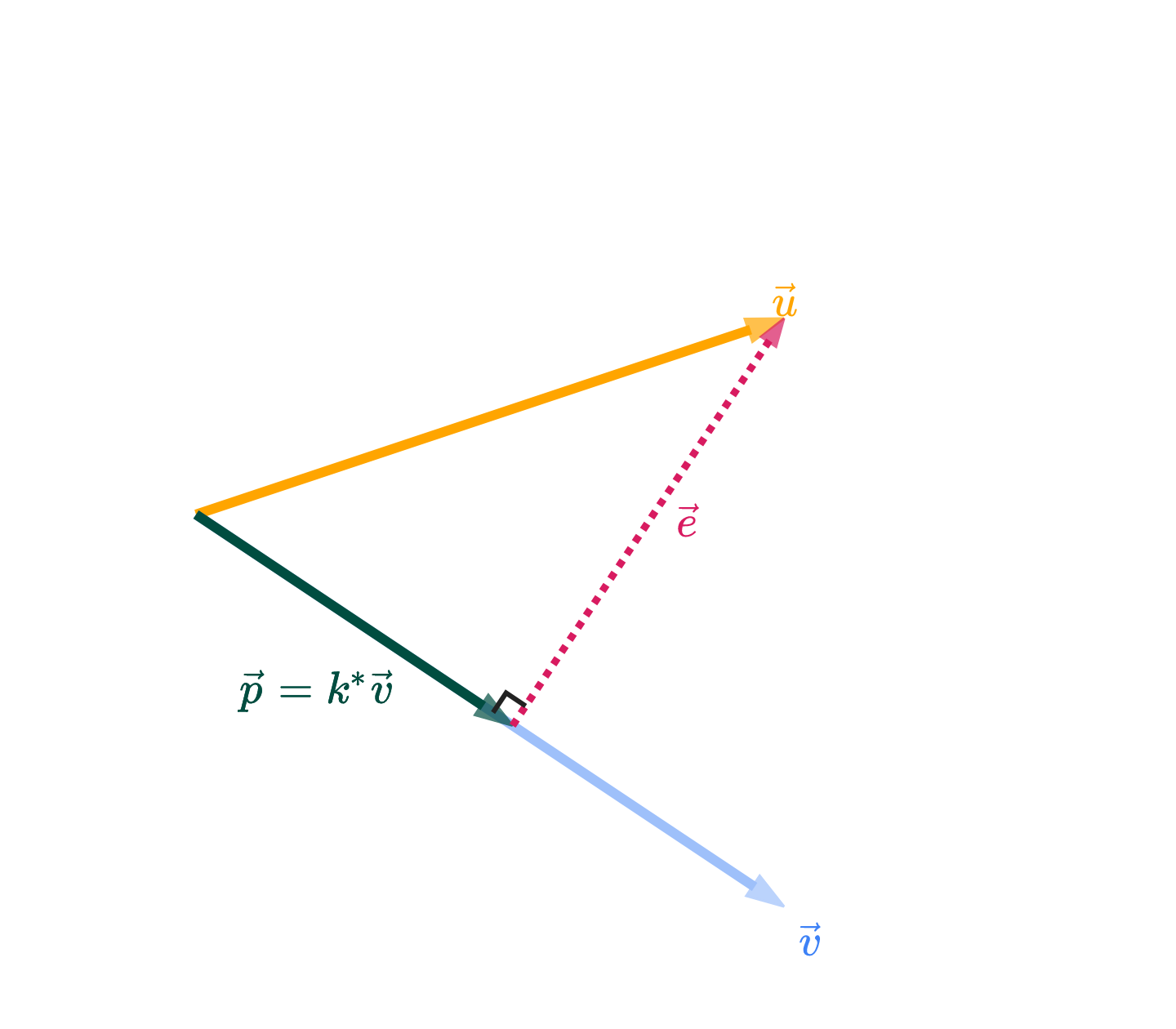
We know that the answer is k∗v, where k∗ is the value of k that makes the error vector e=u−k∗v orthogonal to v. (I’ve switched from calling this optimal scalar ko to k∗; ko was a name I used in the proof above, but more generally, “optimal” values are starred for our purposes).
Let’s now find the value of k∗, in terms of just u and v. If e is orthogonal to v, then v⋅e=0.
The boxed value above is a scalar. It tells us the optimal amount to multiply v by to get the best approximation of u. Once we multiply that boxed scalar, k∗, by the vector v, we get what’s called the orthogonal projection of u onto v.
Among all vectors of the form kv, p above is the one that is closest to u.
Why “orthogonal projection”? “Orthogonal” comes from the fact that p’s error vector e=u−p is orthogonal to v. “Projection” comes from the intuition you should have that p is the shadow of u onto v.
We might say 2/3 is the projection error. Another way of thinking of it is as the shortest distance from the point (1,2,2) to the line that passes through (0,0,0) and (1,1,1).
Consider the points p1=(1,2,2) and p2=(1,1,1) in R3.
What is the shortest distance between p1 and the line that passes through p2 and the origin, (0,0,0)?
Solution
The answer is 2/3. This example didn’t require any addition math beyond the previous example; it just serves to remind you of the geometry of the situation. The set of all possible scalar multiples of v fill out a line in R3, and that line passes through (0,0,0) and p2=(1,1,1).
Why does that line pass through (0,0,0)? Consider the vector 0v – it’s the zero vector!
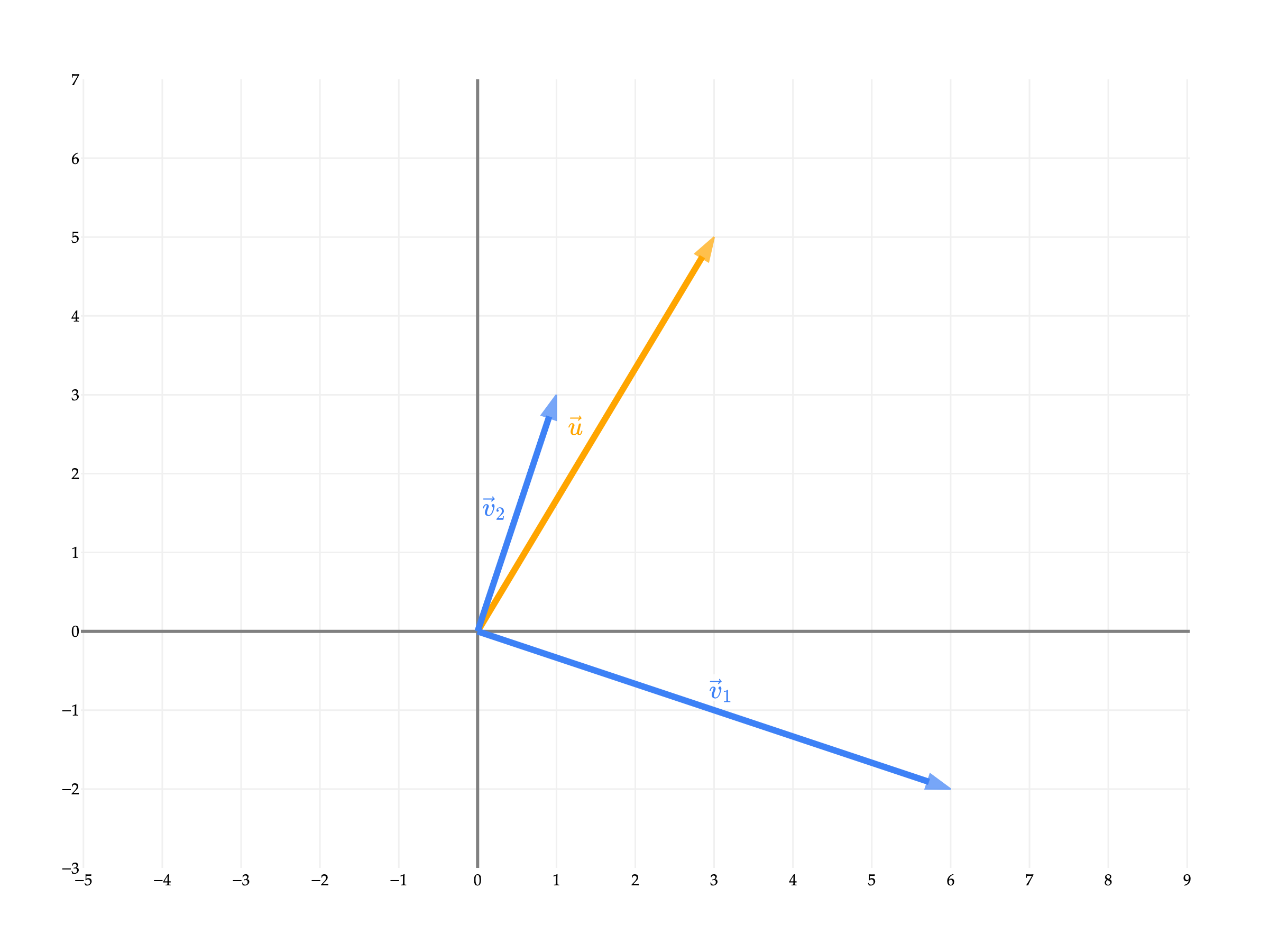
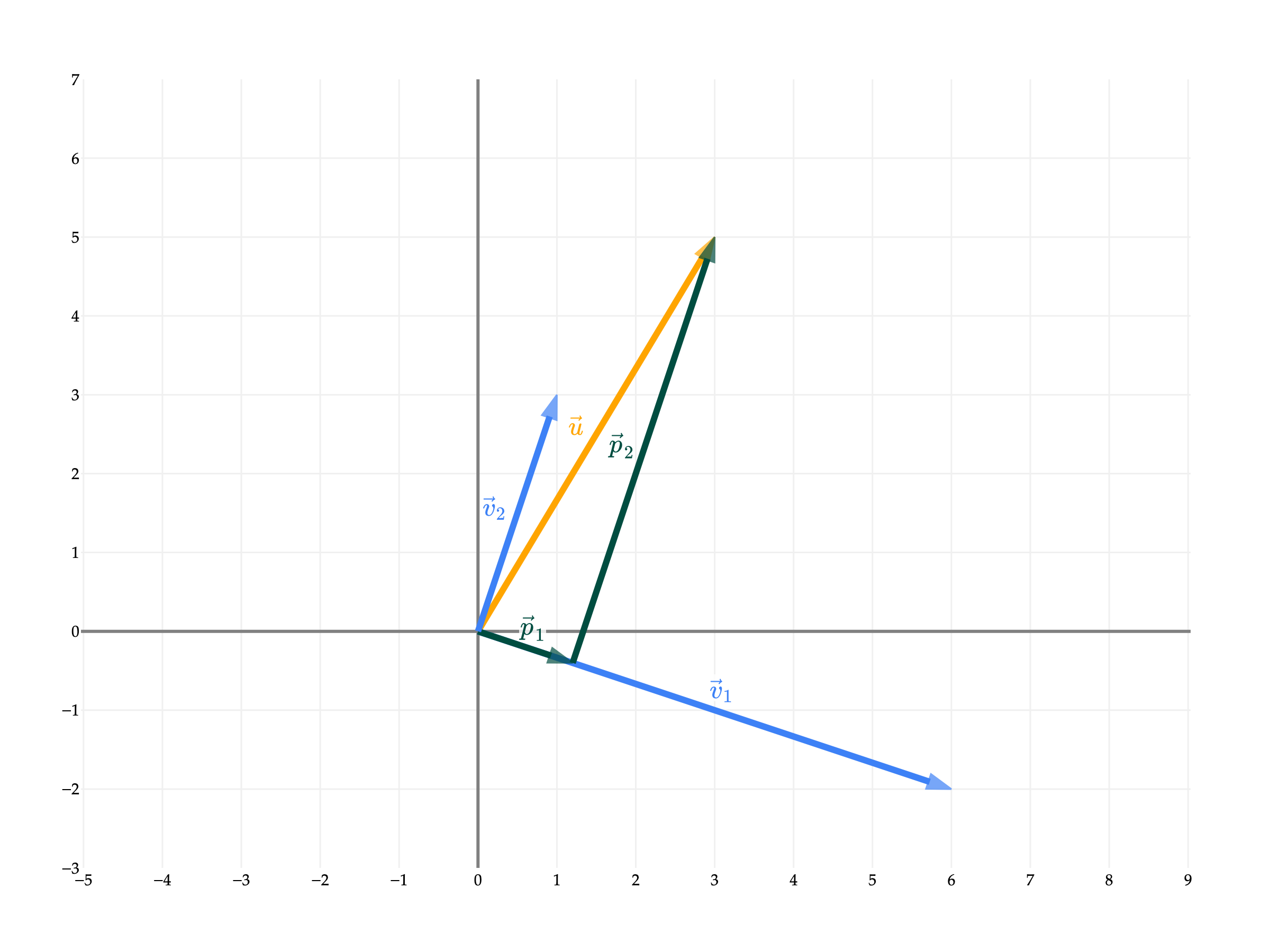
In the first example, we found the orthogonal projection of u onto v.
Now, do the opposite: find the orthogonal projection of v onto u.
Solution
Now, we’re projecting v onto u, which means our answer is going to be a multiple of u, not v as in the first part.
The orthogonal projection of v onto u is given by
p=u⋅uv⋅uu
The formula for the scalar in front of u is the same as in Part 1, but with all v’s replaced by u’s and vice versa. The numerator is the same, since u⋅v=v⋅u. The denominator is different; just remember that the denominator is the squared norm of the vector you’re projecting onto.
v⋅u=⎣⎡111⎦⎤⋅⎣⎡122⎦⎤=1+2+2=5
u⋅u=⎣⎡122⎦⎤⋅⎣⎡122⎦⎤=1+4+4=9
So, the orthogonal projection of v onto u is
p=u⋅uv⋅uu=95⎣⎡122⎦⎤=⎣⎡5/910/910/9⎦⎤
Note that the corresponding error vector, e=v−p, is orthogonal to u (notv), since u is the vector we projected onto.
Notice that in both parts, the orthogonal projection p is the same! This is not a coincidence. Both vectors point in the same direction, meaning the set of possible vectors of the form kV is the same as the set of possible vectors of the form kv. Another way to think about this is that they both span the same line in R3 through the origin.
The difference between v and V is that V is a unit vector in the direction of v, meaning that it points in the same direction as v but has ∥V∥=1 rather than ∥v∥=7.
What’s different is the scalar we need to multiply each vector by to get the orthogonal projection. In the case of the unit vector V, the number in front of V is V⋅Vu⋅V, but since V⋅V=∥V∥2=1, this simplifies to u⋅V.
Suppose u,v∈Rn. Let θ be the angle between u and v.
Show that the orthogonal projection of u onto v is equal to
p=(∥u∥cosθ)∥v∥v
This is not a formula we’d use to actually compute p, since finding cosθ is harder than using the dot product-based formula from above. But, what does this formula tell us about the relationship between u and p?
Solution
Let’s start with the original formula for the orthogonal projection of u onto v.
p=v⋅vu⋅vv
Using the fact that u⋅v=∥u∥∥v∥cosθ and v⋅v=∥v∥2, we can rewrite the formula as
p=∥v∥2∥u∥∥v∥cosθv=∥v∥∥u∥cosθv=(∥u∥cosθ)∥v∥v
The parentheses around ∥u∥cosθ don’t change the calculation, but they help with the interpretation. This shows us that we can think of the orthogonal projection of u onto v as a vector with:
a length of ∥u∥cosθ
in the direction of ∥v∥v, which is a unit vector in the direction of v
u and v are orthogonal. What does this say about the orthogonal projection of u onto v?
Solution
Since u⋅v=0, the orthogonal projection of u onto v is the zero vector, 0.
p=v⋅vu⋅vv=360v=0
Intuitively, u and v travel in totally different different directions. Travelling any amount of v will take you further away from u. So, it’s best to stick with the zero vector, 0.
Why is the sum of p1 and p2 equal to u? Earlier, I mentioned that we can use orthogonal projections to decompose vectors. Here, when we project u onto v1, the corresponding error vector e1 is orthogonal to v1.
u=parallel to v1p1+orthogonal to v1e1
By projecting u onto v2, we can recreate the error vector exactly, meaning e1=p2.
Taking a step back, the fact that v1 and v2 are orthogonal meant that writing u as a linear combination of v1 and v2 was easy.
a1v1[6−2]+a2v2[13]=u[35]
If v1 and v2 were not orthogonal, then writing u as a linear combination of v1 and v2 would have involved solving a system of 2 equations and 2 unknowns, as we’ve had to do in previous sections.
For instance, if we keep [35] and look at x1=[12] and x2=[21], we have that
the projection of u onto x1 is (x1⋅x1u⋅x1)x1=513x1
the projection of u onto x2 is (x2⋅x2u⋅x2)x2=511x2
I’d like to provide a more general “theorem”, on when you can use orthogonal projections to more easily write a vector u as a linear combination of vectors v1, v2, ..., vd, but we’ll need to first study the idea of a basis. That’s to come.
This section has been light on activities, since it provided many examples that we’ll work through in lecture. But, here’s one to tie this last point together.
The motivating problem for this section was the approximation problem, which asked us to find the best approximation of a vector u using only a scalar multiple of a vector v.
The next natural step is to consider the case where we want to approximate u using a linear combination of more than one vector, v1, v2, ..., vd. Why? Remember, this all connects back to the problem of linear regression. The more vectors we have as “building blocks” in our linear combination, the more features our model will be able to use. (I haven’t made the connection from linear algebra to linear regression yet, but just know this is why we’re studying projections.)
For example, let’s consider u=⎣⎡136⎦⎤, v1=⎣⎡101⎦⎤, and v2=⎣⎡221⎦⎤. Among all linear combinations of v1 and v2, which one is closest to u?
To answer this question, we’d need to find the scalars a1 and a2 such that the error vector
e=u−(a1v1+a2v2)
has minimal length, which presumably happens when e is orthogonal to both v1 and v2.
Travelling down this road, we might be able to find the values of a1 and a2 that minimize the length of e. But then we’ll want to ask how we can do this for any u and any set of vectors v1, v2, ..., vd, and it seems like we’ll need a more general solution. In general, to find the “best” approximation of u using a linear combination of v1, v2, ..., vd, we’ll need to know about matrices. We’ll introduce matrices in Chapter 2.5.
Instead, in Chapter 2.4, we will set aside the goal of projections temporarily, and instead focus on truly understanding the set of possible linear combinations of a given set of vectors. For example, the vectors v1=⎣⎡100⎦⎤, v2=⎣⎡−518⎦⎤ from earlier define a plane. So, asking which linear combination of v1 and v2 is closest to u is equivalent to asking which point on the plane is closest to u.
from utils import plot_vectors
import numpy as np
import plotly.graph_objects as go

# Define the vectors
u = (1, 3, 6)
v1 = (1, 0, 1)
v2 = (2, 2, 1)

# Plot the vectors using plot_vectors function
vectors = [
    (u, "orange", r"u"),
    (v1, "#3d81f6", r"v₁"),
    (v2, "#3d81f6", r"v₂"),
]

fig = plot_vectors(vectors, show_axis_labels=True, vdeltay=1)

# Make the plane look more rectangular by using a smaller, symmetric range for s and t
plane_extent = 20  # controls the "size" of the rectangle
num_points = 3   # fewer points for a cleaner rectangle

s_range = np.linspace(-plane_extent, plane_extent, num_points)
t_range = np.linspace(-plane_extent, plane_extent, num_points)
s_grid, t_grid = np.meshgrid(s_range, t_range)

plane_x = s_grid * v1[0] + t_grid * v2[0]
plane_y = s_grid * v1[1] + t_grid * v2[1]
plane_z = s_grid * v1[2] + t_grid * v2[2]

fig.add_trace(go.Surface(
    x=plane_x,
    y=plane_y,
    z=plane_z,
    opacity=0.8,
    colorscale=[[0, 'rgba(61,129,246,0.3)'], [1, 'rgba(61,129,246,0.3)']],
    showscale=False,
))

fig.update_layout(
    scene_camera=dict(
        eye=dict(x=0.8, y=2, z=1.2)
    ),
    scene=dict(
        zaxis=dict(range=[-3, 4])  # ensure z-axis hits -3
    ),
)

fig.show()
Loading...
Chapter 2.4 will answer the questions, “why do v1 and v2 define a plane?”, “which plane do they define?”, and “in general, what do v1, v2, ..., vd, all in Rn, define?”