2.2. The Dot Product - Math for ML Course Notes

Definitions¶

In Chapter 2.1, we learned how to add and scale vectors. The next natural operation is to consider how to multiply two vectors together. Let’s start with a definition, and then make sense of it.

The Computational Definition¶

Definition: Dot Product

Suppose ${\color{orange} \vec u}, {\color{#3d81f6} \vec v} \in \mathbb{R}^n$ , i.e. both are vectors with $n$ components.

Then, the dot product of ${\color{orange} \vec u}$ and ${\color{#3d81f6} \vec v}$ , denoted by ${\color{orange} \vec u} \cdot {\color{#3d81f6} \vec v}$ , is the scalar defined as follows:

{\color{orange} \vec u} \cdot {\color{#3d81f6} \vec v} = {\color{orange} \begin{bmatrix} u_1 \\ u_2 \\ \vdots \\ u_n \end{bmatrix}} \cdot {\color{#3d81f6} \begin{bmatrix} v_1 \\ v_2 \\ \vdots \\ v_n \end{bmatrix}} = {\color{orange} u_1} {\color{#3d81f6} v_1} + {\color{orange} u_2} {\color{#3d81f6} v_2} + \cdots + {\color{orange} u_n} {\color{#3d81f6} v_n}

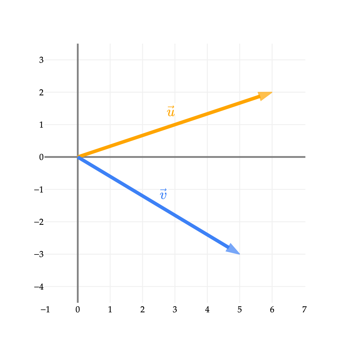
I call this the computational definition because it’s the definition that’s easiest to compute. Let’s work out an example. Consider the vectors $\color{orange} \vec u = \begin{bmatrix} 6 \\ 2 \end{bmatrix}$ and $\color{#3d81f6} \vec v = \begin{bmatrix} 5 \\ -3 \end{bmatrix}$ . Their dot product is:

{\color{orange} \vec u} \cdot {\color{#3d81f6} \vec v} = {\color{orange} \begin{bmatrix} 6 \\ 2 \end{bmatrix}} \cdot {\color{#3d81f6} \begin{bmatrix} 5 \\ -3 \end{bmatrix}} = ({\color{orange} 6}) ({\color{#3d81f6} 5}) + ({\color{orange} 2}) ({\color{#3d81f6} -3}) = 30 - 6 = 24

Note that the dot product is one number (24 here), not another vector.

Activity 1

Activity 1.1

Let $\vec z = \begin{bmatrix} 5 \\ 3 \\ -1 \end{bmatrix}$ and $\vec 1 = \begin{bmatrix} 1 \\ 1 \\ 1 \end{bmatrix}$ .

Find $\vec z \cdot \vec 1$ .
In general, if $z \in \mathbb{R}^n$ is any vector, and $\vec 1 = \begin{bmatrix} 1 \\ 1 \\ \vdots \\ 1 \end{bmatrix}$ is a vector of all 1s with the same number of components as $\vec z$ , what is the value of:

\vec z \cdot 1

Activity 1.2

Dot products are useful for computing weighted averages. Let’s illustrate that here. In your freshman fall semester, you took the following courses and earned the following grades:

Course	Grade	Credits
EECS 245	4 (A+)	4
MATH 116	3.7 (A-)	3
EECS 201	0 (F)	1
DATASCI 101	3.3 (B+)	4

Find your GPA for the semester, and express it as a dot product between a grades vector $\vec g$ and a weights vector $\vec w$ .

What does the dot product of 24 tell us about $\color{orange} \vec u$ and $\color{#3d81f6} \vec v$ ?

# This chunk must be in the first plotting cell of each notebook in order to guarantee that the mathjax script is loaded.

import plotly
from IPython.display import display, HTML

plotly.offline.init_notebook_mode()
plotly.io.renderers.default = "png"
display(HTML(
    '<script type="text/javascript" async src="https://cdnjs.cloudflare.com/ajax/libs/mathjax/2.7.1/MathJax.js?config=TeX-MML-AM_SVG"></script>'
))

# ---

from utils import plot_vectors
import numpy as np

fig = plot_vectors([((6, 2), 'orange', r'$\vec u$'), ((5, -3), '#3d81f6', r'$\vec v$')],
                   vdeltax=0.3, vdeltay=0.5)
fig.update_layout(width=400, height=400, yaxis_scaleanchor="x")
fig.update_xaxes(range=[-1, 7], tickvals=np.arange(-4, 10))
fig.update_yaxes(range=[-4, 3], tickvals=np.arange(-4, 4))
fig.show(scale=3)

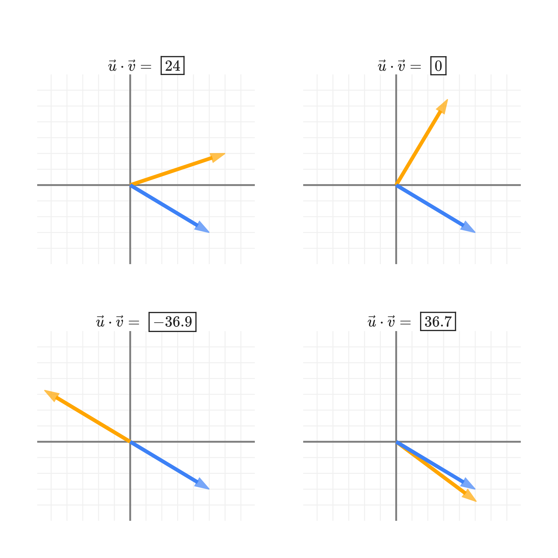
On its own, 24 doesn’t mean much. Let’s imagine we keep $\color{#3d81f6} \vec v$ fixed, and move $\color{orange} \vec u$ around. What do you notice about the resulting dot products?

from utils import plot_vectors
import numpy as np
import plotly.graph_objects as go
from plotly.subplots import make_subplots

# Original vectors
v = np.array([5, -3])
u_original = np.array([6, 2])

# Calculate norm of original u
u_norm = np.sqrt(np.sum(u_original**2))  # sqrt(40)

# Define the four different u vectors
u_vectors = []

# Top left: original u
u1 = u_original
u_vectors.append((u1, "Original u"))

# Top right: perpendicular to v with same norm
perp_v = np.array([3, 5])  # perpendicular to v
u2 = perp_v * (u_norm / np.linalg.norm(perp_v))
u_vectors.append((u2, "u ⊥ v"))

# Bottom left: u = (6, 2)
u3 = np.array([-5, 3]) * u_norm / np.linalg.norm(np.array([-5, 3]))
u_vectors.append((u3, "u = (-5, 3)"))

# Bottom right: slightly more negative than v but close to v
v_normalized = v / np.linalg.norm(v)
angle_offset = -0.1  # small negative angle offset
cos_offset = np.cos(angle_offset)
sin_offset = np.sin(angle_offset)
rotation_matrix = np.array([[cos_offset, -sin_offset], [sin_offset, cos_offset]])
u4_direction = rotation_matrix @ v_normalized
u4 = u4_direction * u_norm
u_vectors.append((u4, "u close to v"))

# Create subplots
fig = make_subplots(
    rows=2, cols=2,
    subplot_titles=[r"$\vec u \cdot \vec v =" f"\\boxed{{{np.dot(u, v):.1f}}}$".replace('-0.0', '0').replace('.0', '') for u, _ in u_vectors],
    horizontal_spacing=0.1,
    vertical_spacing=0.15
)

positions = [(1, 1), (1, 2), (2, 1), (2, 2)]

# Define consistent axis settings for perfect squares
axis_range = [-5, 7]
tick_spacing = 1
axis_ticks = np.arange(axis_range[0], axis_range[1] + 1, tick_spacing)

for i, ((u, description), (row, col)) in enumerate(zip(u_vectors, positions)):
    temp_fig = plot_vectors([
        (tuple(u), 'orange', r'$\vec u$'), 
        (tuple(v), '#3d81f6', r'$\vec v$')
    ], vdeltax=0.3, vdeltay=0.5)
    for trace in temp_fig.data:
        fig.add_trace(trace, row=row, col=col)

# Apply consistent axis settings to all subplots for perfect squares
for row in range(1, 3):
    for col in range(1, 3):
        fig.update_xaxes(
            range=axis_range, 
            tickvals=axis_ticks,
            showticklabels=False,
            showgrid=True,
            gridcolor="#f0f0f0",
            zeroline=True,
            zerolinecolor="gray",
            mirror=True,
            ticks="",
            tickfont=dict(family="Palatino", size=14),
            title_font=dict(family="Palatino", size=16),
            row=row, col=col
        )
        fig.update_yaxes(
            range=axis_range, 
            tickvals=axis_ticks,
            showticklabels=False,
            showgrid=True,
            gridcolor="#f0f0f0",
            zeroline=True,
            zerolinecolor="gray",
            mirror=True,
            ticks="",
            tickfont=dict(family="Palatino", size=14),
            title_font=dict(family="Palatino", size=16),
            scaleanchor=f"x{row}{col}" if row == 1 and col == 1 else f"x{row}{col}",
            row=row, col=col
        )

fig.update_layout(
    width=600,
    height=600,
    showlegend=False,
    font=dict(family="Palatino", size=16, color="#222"),
    paper_bgcolor="white",
    plot_bgcolor="white",
    margin=dict(l=40, r=40, t=80, b=40)
)

# Ensure equal aspect ratio for perfect squares
fig.update_yaxes(scaleanchor="x", scaleratio=1, row=1, col=1)
fig.update_yaxes(scaleanchor="x2", scaleratio=1, row=1, col=2)
fig.update_yaxes(scaleanchor="x3", scaleratio=1, row=2, col=1)
fig.update_yaxes(scaleanchor="x4", scaleratio=1, row=2, col=2)

fig.show(scale=3)

It seems like the dot product has something to do with the angle between $\color{orange} \vec u$ and $\color{#3d81f6} \vec v$ :

When $\color{orange} \vec u \cdot \color{#3d81f6} \vec v$ is large and positive, it seems like the two vectors are pointing in the same direction. (The larger the dot product, the more aligned they are.)
When $\color{orange} \vec u \cdot \color{#3d81f6} \vec v$ is large and negative, it seems like the two vectors are pointing in opposite directions.
When $\color{orange} \vec u \cdot \color{#3d81f6} \vec v$ is 0, it seems like the two vectors are perpendicular.

In fact, there’s another equivalent definition of the dot product that makes this relationship explicit.

The Geometric Definition¶

Activity 2

The fact that the two definitions of the dot product are equivalent allows us to use the dot product to find the angle between two vectors.

Let $\vec w = \begin{bmatrix} 5 \\ 0 \\ -4 \end{bmatrix}$ and $\vec x = \begin{bmatrix} 9 \\ 1 \\ 2 \end{bmatrix}$ .

Find the dot product between $\vec w$ and $\vec x$ .
Find the angle between $\vec w$ and $\vec x$ . Leave your answer in the form $\cos^{-1} ( \cdot )$ .

Solution

$\vec w \cdot \vec x = \begin{bmatrix} 5 \\ 0 \\ -4 \end{bmatrix} \cdot \begin{bmatrix} 9 \\ 1 \\ 2 \end{bmatrix} = 5 \cdot 9 + 0 \cdot 1 + (-4) \cdot 2 = 45 - 8 = 37$ .
Since $\vec w \cdot \vec x = 37$ , and $\vec w \cdot \vec x = \left\| \vec w \right\| \left\| \vec x \right\| \cos \theta$ , we have

\begin{align*}37 &= \lVert \vec w \rVert \lVert \vec x \rVert \cos \theta \\ \implies \cos \theta &= \frac{37}{\lVert \vec w \rVert \lVert \vec x \rVert} \\ &= \frac{37}{\sqrt{5^2 + 0^2 + (-4)^2} \sqrt{9^2 + 1^2 + 2^2}} \\ &= \frac{37}{\sqrt{41} \sqrt{86}} \\ \implies \theta &= \cos^{-1} \left( \frac{37}{\sqrt{41} \sqrt{86}} \right)\end{align*}

To prove why these two definitions are equivalent, we’ll need to learn a bit more about the properties of the dot product. For now, let’s just try and interpret this new formula. Here are both definitions of the dot product, for two vectors $\color{orange} \vec u$ and $\color{#3d81f6} \vec v$ :

\begin{aligned} {\color{orange} \vec u} \cdot {\color{#3d81f6} \vec v} &= {\color{orange} u_1} {\color{#3d81f6} v_1} + {\color{orange} u_2} {\color{#3d81f6} v_2} + \cdots + {\color{orange} u_n} {\color{#3d81f6} v_n} \\ &= \left\| {\color{orange} \vec u} \right\| \left\| {\color{#3d81f6} \vec v} \right\| \cos \theta \end{aligned}

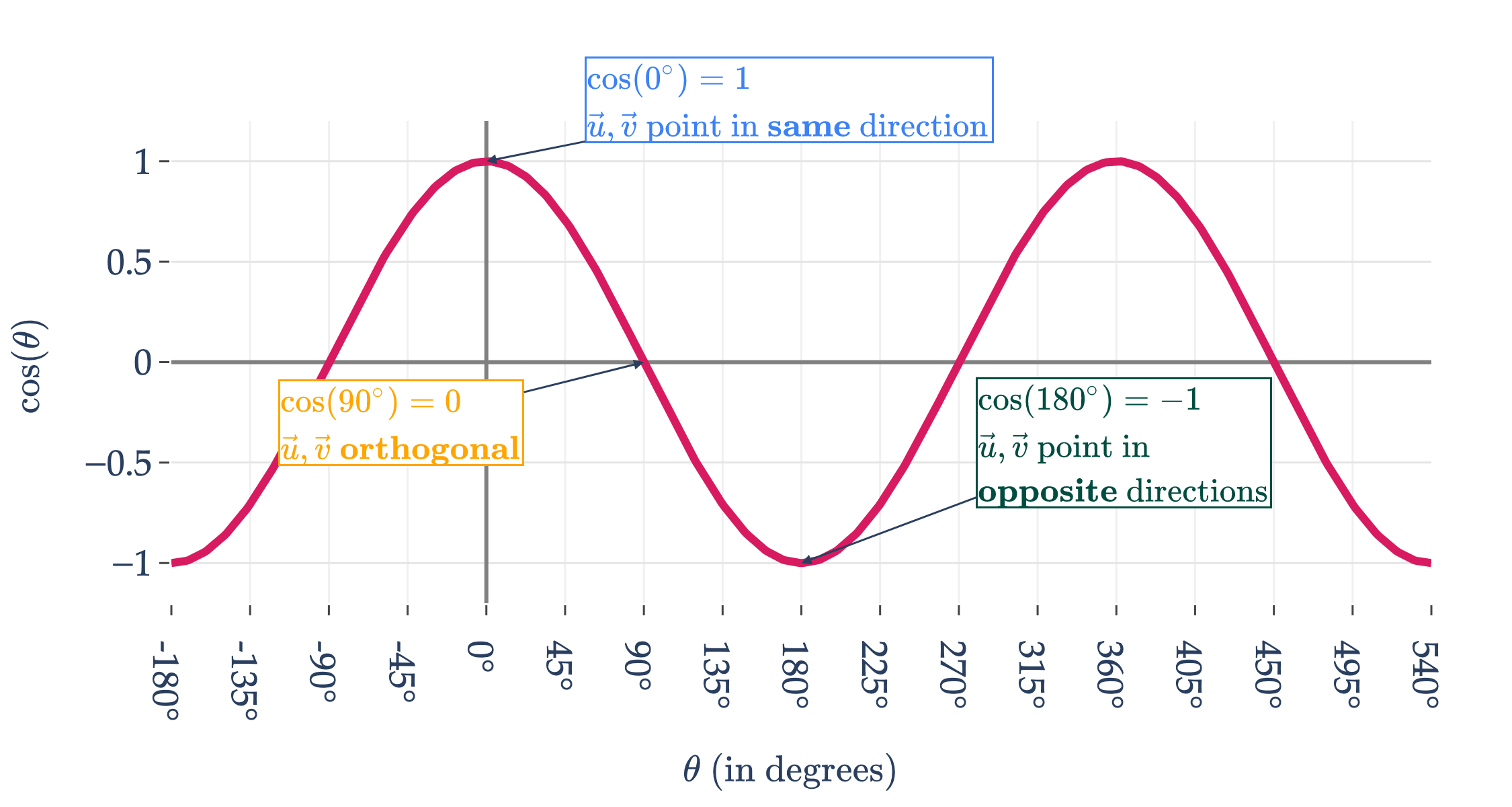
How does the function $\cos \theta$ behave? Remember, $\theta$ is the angle between the two vectors.

import numpy as np
import plotly.graph_objects as go

theta = np.linspace(-180, 540, 500)
y = np.cos(np.deg2rad(theta))

fig = go.Figure()

fig.add_trace(go.Scatter(
    x=theta,
    y=y,
    mode='lines',
    line=dict(color='#d81b60', width=4),
    name='y = cos(θ)'
))

# Add intuitive annotations at cos = 1, 0, -1
fig.add_annotation(
    x=0, y=1,
    text=r"$\cos(0^\circ) = 1 \\ \vec u, \vec v \text{ point in} \textbf{ same} \text{ direction}$",
    showarrow=True,
    arrowhead=2,
    ax=150, ay=-30,
    font=dict(size=16, color="#3d81f6"),
    bgcolor="white",
    bordercolor="#3d81f6",
)
fig.add_annotation(
    x=90, y=0,
    text=r"$\cos(90^\circ) = 0 \\ \vec u, \vec v  \textbf{ orthogonal}$",
    showarrow=True,
    arrowhead=2,
    ax=-120, ay=30,
    font=dict(size=16, color="orange"),
    bgcolor="white",
    bordercolor="orange",
)
fig.add_annotation(
    x=180, y=-1,
    text=r"$\cos(180^\circ) = -1 \\ \vec u, \vec v \text{ point in} \\ \textbf{opposite} \text{ directions}$",
    showarrow=True,
    arrowhead=2,
    ax=160, ay=-60,
    font=dict(size=16, color="#004d40"),
    bgcolor="white",
    bordercolor="#004d40",
)

fig.update_layout(
    font=dict(family='Palatino, serif', size=18),
    xaxis=dict(
        title=r'$\theta \text{ (in degrees)}$',
        gridcolor='#f0f0f0',
        zerolinecolor='gray',
        # linecolor='#bbbbbb',
        mirror=True,
        ticks='outside',
        showline=True,
        tickvals=np.arange(-180, 540 + 45, 45),
        ticktext=["-180°", "-135°", "-90°", "-45°", "0°", "45°", "90°", "135°", "180°", "225°", "270°", "315°", "360°", "405°", "450°", "495°", "540°"],
    ),
    yaxis=dict(
        title=r'$\cos(\theta)$',
        gridcolor='#e5e5e5',
        zerolinecolor='gray',
        # linecolor='#bbbbbb',
        mirror=True,
        ticks='outside',
        showline=True,
        range=[-1.2, 1.2]
    ),
    plot_bgcolor='white',
    paper_bgcolor='white',
    width=750,
    height=400,
    margin=dict(l=40, r=40, t=60, b=40)
)

fig.show(scale=3)

This explains what we saw in the earlier grid, which contained four pairs of vectors along with their dot products. To recap the logic:

\substack{\text{two vectors point} \\ \text{in similar directions}} \implies \theta \text{ small} \implies \cos \theta \text{ close to 1} \implies \text{dot product large}

There’s another hugely important property that the plot of $\cos \theta$ reveals. Hugely.

Orthogonal Vectors¶

Orthogonal is just a fancy word for perpendicular. Both words mean that the two vectors are at a right angle (90º) to each other.

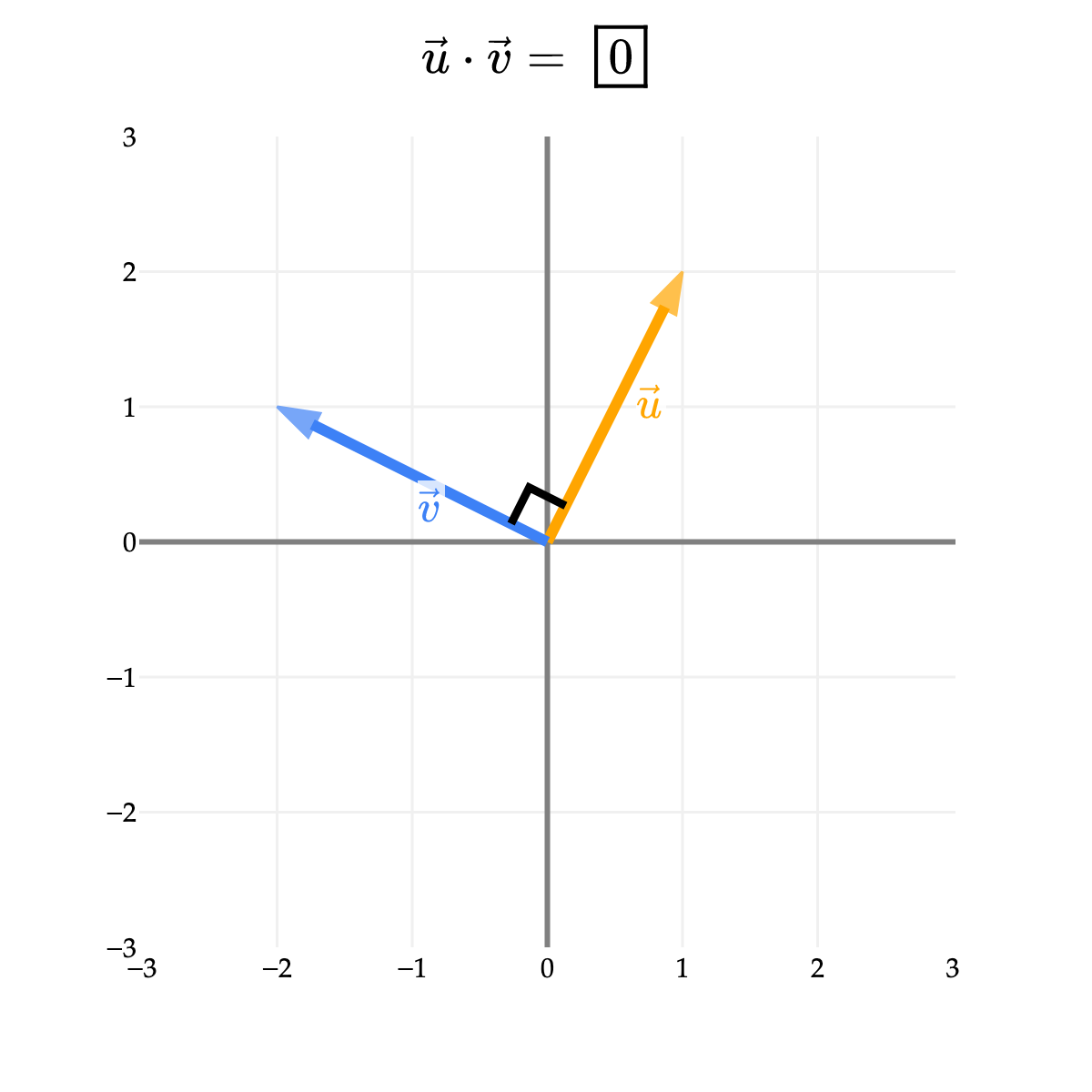
As an example in $\mathbb{R}^2$ , the vectors $\color{orange} \vec u = \begin{bmatrix} 1 \\ 2 \end{bmatrix}$ and $\color{#3d81f6} \vec v = \begin{bmatrix} -10 \\ 5 \end{bmatrix}$ are orthogonal:

Computationally, ${\color{orange} \vec u} \cdot {\color{#3d81f6} \vec v} = ({\color{orange} 1})({\color{#3d81f6} -10}) + ({\color{orange} 2})({\color{#3d81f6} 5}) = -10 + 10 = 0$ .
Geometrically, the angle between them is 90 degrees, so $\cos \theta = 0$ , meaning ${\color{orange} \vec u} \cdot {\color{#3d81f6} \vec v} = {\color{orange}\left\| \vec u \right\|} {\color{#3d81f6} \left\| \vec v \right\|} \cos \theta = 0$ .

from utils import plot_vectors
import numpy as np

fig = plot_vectors([((1, 2), 'orange', r'$\vec u$'), ((-2, 1), '#3d81f6', r'$\vec v$')],
                   vdeltax=-0.3, vdeltay=0.2)

# Add a right angle annotation between u and v
# Vectors u = (1, 2) and v = (-2, 1)
u = np.array([1, 2])
v = np.array([-2, 1])

# Normalize the vectors and scale them for the right angle marker
scale = 0.3  # Size of the right angle marker
u_norm = u / np.linalg.norm(u) * scale
v_norm = v / np.linalg.norm(v) * scale

# Create the right angle marker by drawing a small square
# Starting from origin, go along u_norm, then along v_norm, then back
fig.add_shape(
    type="path",
    path=f"M {u_norm[0]} {u_norm[1]} L {u_norm[0] + v_norm[0]} {u_norm[1] + v_norm[1]} L {v_norm[0]} {v_norm[1]}",
    line=dict(color="black", width=3),
    layer="above",
)

fig.update_layout(width=400, height=400, yaxis_scaleanchor="x", title=r"$\vec u \cdot \vec v = \boxed{0}$", title_x=0.5)
fig.update_xaxes(range=[-3, 3], tickvals=np.arange(-4, 10))
fig.update_yaxes(range=[-3, 3], tickvals=np.arange(-4, 8))
fig.show(config={'displayModeBar': False}, renderer='png', scale=3)

For an example in $\mathbb{R}^3$ , the vectors $\color{#d81b60} \vec w = \begin{bmatrix} 3 \\ 6 \\ 2 \end{bmatrix}$ and $\color{#004d40} \vec r = \begin{bmatrix} -5 \\ 2 \\ \frac{3}{2} \end{bmatrix}$ are also orthogonal:

Computationally, ${\color{#d81b60} \vec w} \cdot {\color{#004d40} \vec r} = ({\color{#d81b60} 3})({\color{#004d40} -5}) + ({\color{#d81b60} 6})({\color{#004d40} 2}) + ({\color{#d81b60} 2})({\color{#004d40} \frac{3}{2}}) = -15 + 12 + 3 = 0$ .
Geometrically, the angle between them is 90 degrees, so $\cos \theta = 0$ , meaning ${\color{#d81b60} \vec w} \cdot {\color{#004d40} \vec r} = {\color{#d81b60} \left\| \vec w \right\|} {\color{#004d40} \left\| \vec r \right\|} \cos \theta = 0$ .

from utils import plot_vectors
import numpy as np

fig = plot_vectors([((3, 6, 2), '#d81b60', r'<b>w</b>'), ((-5, 2, 1.5), '#004d40', r'<b>r</b>')],
                   vdeltax=-1, vdeltay=1)

# Add a right angle annotation between w and r vectors
# Vectors w = (3, 6, 2) and r = (-5, 2, 1.5)
w = np.array([3, 6, 2])
r = np.array([-5, 2, 1.5])

# Normalize the vectors and scale them for the right angle marker
scale = 1.0  # Size of the right angle marker
w_norm = w / np.linalg.norm(w) * scale
r_norm = r / np.linalg.norm(r) * scale

# Create the right angle marker by drawing a small square
# Starting from origin, go along w_norm, then along r_norm, then back
fig.add_scatter3d(
    x=[0, w_norm[0], w_norm[0] + r_norm[0], r_norm[0], 0],
    y=[0, w_norm[1], w_norm[1] + r_norm[1], r_norm[1], 0],
    z=[0, w_norm[2], w_norm[2] + r_norm[2], r_norm[2], 0],
    mode='lines',
    line=dict(color='black', width=4),
    showlegend=False,
    name='Right Angle'
)

# Make all grid boxes the same size (cubes) by setting equal aspect ratio
# and matching ranges for all three axes - zoomed in to relevant region
axis_range = [-6, 7]
tick_values = np.arange(-6, 8, 2)

fig.update_layout(
    width=500, 
    height=500,
    title=r"$\vec w \cdot \vec r = \boxed{0}$", 
    title_x=0.5,
    title_y=0.9,
    scene=dict(
        xaxis=dict(
            range=axis_range,
            tickvals=tick_values,
            nticks=10,
            showgrid=True,
            gridwidth=1,
            gridcolor='lightgray'
        ),
        yaxis=dict(
            range=axis_range,
            tickvals=tick_values,
            nticks=10,
            showgrid=True,
            gridwidth=1,
            gridcolor='lightgray'
        ),
        zaxis=dict(
            range=axis_range,
            tickvals=tick_values,
            nticks=10,
            showgrid=True,
            gridwidth=1,
            gridcolor='lightgray'
        ),
        aspectmode='cube',  # This ensures all axes have equal scaling
        camera=dict(
            eye=dict(x=1, y=0.5, z=2.5)  # High z viewpoint to see orthogonality from above
        )
    )
)

fig.show(config={'displayModeBar': False}, renderer='notebook')

What does a right angle look like in 4 or higher dimensions? I’m not sure, but that’s the beauty of abstraction once again – this definition of orthogonality works in any dimension, just like our definitions of the dot product. If two vectors are orthogonal, I like thinking of them as being “as different as possible”, in contrast to two vectors that point in the same direction.

Orthogonality, as it turns out, is crucial to our goal of framing the linear regression problem in terms of linear algebra. I’m not a big proponent of asking you to memorize things (I’d rather you internalize them through practice!), but the definition of orthogonality is one that you need to remember.

Activity 3

Activity 3.1

Find a value of $k$ such that the vectors $\vec u = \begin{bmatrix} 9 \\ -2 \\ 1 \end{bmatrix}$ and $\vec v = \begin{bmatrix} 1 \\ k \\ 3 \end{bmatrix}$ are orthogonal.

Is this value of $k$ unique?

Activity 3.2

Find a vector that is orthogonal to both $\vec u = \begin{bmatrix} 1 \\ -2 \\ 4 \end{bmatrix}$ and $\vec v = \begin{bmatrix} 3 \\ -1 \\ 9 \end{bmatrix}$ . In $\mathbb{R}^3$ , what does this new vector look like, relative to $\vec u$ and $\vec v$ ?

Properties of the Dot Product¶

Properties of the Dot Product

Recall, for any vectors ${\color{orange} \vec u}, {\color{#3d81f6} \vec v} \in \mathbb{R}^n$ , the dot product is defined as:

\begin{aligned} {\color{orange} \vec u} \cdot {\color{#3d81f6} \vec v} &= {\color{orange} u_1} {\color{#3d81f6} v_1} + {\color{orange} u_2} {\color{#3d81f6} v_2} + \cdots + {\color{orange} u_n} {\color{#3d81f6} v_n} \\ &= \left\| {\color{orange} \vec u} \right\| \left\| {\color{#3d81f6} \vec v} \right\| \cos \theta \end{aligned}

The dot product satisfies the following properties:

Commutative property: ${\color{orange} \vec u} \cdot {\color{#3d81f6} \vec v} = {\color{#3d81f6} \vec v} \cdot {\color{orange} \vec u}$
Distributive property: ${\color{orange} \vec u} \cdot ({\color{#3d81f6} \vec v} + {\color{#d81b60} \vec w}) = {\color{orange} \vec u} \cdot {\color{#3d81f6} \vec v} + {\color{orange} \vec u} \cdot {\color{#d81b60} \vec w}$
Associative property with respect to a scalar: ${\color{orange} c} ({\color{#3d81f6} \vec v} \cdot {\color{#d81b60} \vec w}) = ({\color{orange} c} {\color{#3d81f6} \vec v}) \cdot {\color{#d81b60} \vec w} = {\color{#3d81f6} \vec v} \cdot ({\color{orange} c} {\color{#d81b60} \vec w})$

We’ve already taken the commutative property for granted (the angle between $\color{orange} \vec u$ and $\color{#3d81f6} \vec v$ is the same as the angle between $\color{#3d81f6} \vec v$ and $\color{orange} \vec u$ ), and we’re about to see a powerful application of the distributive property (though it’s a good exercise to see if you can verify it yourself).

Let me comment on the last property, the associativity of the dot product with respect to a scalar. In standard multiplication, the associativity property for scalars $a, b, c \in \mathbb{R}$ says that $abc = (ab)c = a(bc)$ . However, this does not hold for the dot product, because the dot product of three vectors has no meaning! Instead, the modified associativity property for the dot product concerns itself with two vectors and a scalar.

Activity 4

Suppose the dot product of $\vec x$ and $\vec y$ is 10, and the angle between $\vec x$ and $\vec y$ is 30º.

What is the dot product of $2 \vec x$ and $3\vec y$ ?
What is the angle between $2 \vec x$ and $3 \vec y$ ?
What is the angle between $2 \vec x$ and $-3 \vec y$ ?

Dot Product and the Vector Norm¶

What is the dot product of a vector with itself? If ${\color{#3d81f6} \vec v} \in \mathbb{R}^n$ , then:

\begin{aligned} \color{#3d81f6} \vec v \cdot \color{#3d81f6} \vec v &= {\color{#3d81f6} v_1} {\color{#3d81f6} v_1} + {\color{#3d81f6} v_2} {\color{#3d81f6} v_2} + \cdots + {\color{#3d81f6} v_n} {\color{#3d81f6} v_n} \\ &= {\color{#3d81f6} v_1}^2 + {\color{#3d81f6} v_2}^2 + \cdots + {\color{#3d81f6} v_n}^2 \\ &= \left\| {\color{#3d81f6} \vec v} \right\|^2 \end{aligned}

The fact that $\boxed{\vec v \cdot \vec v = \left\| \vec v \right\|^2}$ unlocks a variety of powerful analyses, and it’s such a core definition that I’ve boxed it.

For example, we now have the tools to prove that the geometric cosine definition of the dot product is equal to the computational definition! Let’s try and show that:

{\color{orange} u_1} {\color{#3d81f6} v_1} + {\color{orange} u_2} {\color{#3d81f6} v_2} + \cdots + {\color{orange} u_n} {\color{#3d81f6} v_n} = \left\| {\color{orange} \vec u} \right\| \left\| {\color{#3d81f6} \vec v} \right\| \cos \theta

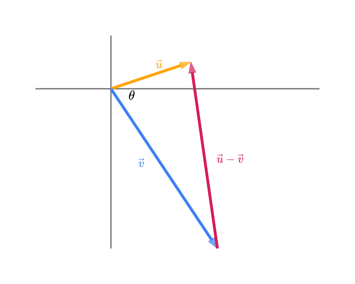
Let’s consider two arbitrary vectors in $\mathbb{R}^n$ , $\color{orange} \vec u$ and $\color{#3d81f6} \vec v$ . (I’ve drawn them below as vectors in $\mathbb{R}^2$ , but we won’t assume anything in particular about two dimensional space, and we won’t put specific numbers to them, since our proof should be general.)

Along with them, let’s consider their difference, $\color{#d81b60} \vec u - \vec v$ . This step may seem arbitrary, but we’ll see why it’s useful soon.

from utils import plot_vectors_non_origin
import numpy as np

u = np.array([3, 1])
v = np.array([4, -6])

# Add an annotation for the angle theta between u and v
fig = plot_vectors_non_origin([(((0, 0), tuple(u)), 'orange', r'$\vec u$'),
                               (((0, 0), tuple(v)), '#3d81f6', r'$\vec v$'),
                               ((tuple(v), tuple(u)), '#d81b60', r'$\vec u - \vec v$')
                               ]
                               , vdeltax=-1, vdeltay=0.5)
fig.update_layout(width=500, height=400, yaxis_scaleanchor="x")
fig.update_xaxes(range=[-1, 6], tickvals=np.arange(-5, 15))
fig.update_yaxes(range=[-8, 4], tickvals=np.arange(-8, 4))

# Calculate a point near the origin for the theta label
theta_label_x = 0.8
theta_label_y = -0.2
fig.add_annotation(
    x=theta_label_x,
    y=theta_label_y,
    text=r'$\theta$',
    showarrow=False,
    font=dict(size=20)
)

fig.update_xaxes(zeroline=True, showticklabels=False, showgrid=False, range=[2, 3])
fig.update_yaxes(zeroline=True, showticklabels=False, showgrid=False, range=[-6, 2])
fig.update_layout(width=500, height=400)
fig.show(scale=3)

A confusing concept is whether the tip of the vector $\color{#d81b60} \vec u - \vec v$ should be at the tip of $\color{orange} \vec u$ or the tip of $\color{#3d81f6} \vec v$ . To verify that the above diagram is correct, note that if you walk along the length of $\color{#3d81f6} \vec v$ , then along the length of $\color{#d81b60} \vec u - \vec v$ , you end up at the tip of $\color{orange} \vec u$ , which matches what we’d expect from the expression ${\color{#3d81f6} \vec v} + ({\color{orange} \vec u} - {\color{#3d81f6} \vec v}) = {\color{orange} \vec u}$ .

I’d like to try and find an expression involving $\theta$ (the angle between $\color{orange} \vec u$ and $\color{#3d81f6} \vec v$ ) and the dot product of $\color{orange} \vec u$ and $\color{#3d81f6} \vec v$ , without using the cosine definition of the dot product (since that’s what I’m trying to prove).

First, let’s consider a rule we perhaps haven’t touched in a few years: the cosine law. The cosine law says that for any triangle with sides of length $a$ , $b$ , and $c$ , with an angle of $C$ opposite side $c$ ,
$\begin{align*} c^2 &= a^2 + b^2 - 2ab \cos C \end{align*}$
We can apply this rule to the triangle formed by $\color{orange} \vec u$ , $\color{#3d81f6} \vec v$ , and $\color{#d81b60} \vec u - \vec v$ (the dashed line in the diagram above). The cosine law tells us that
$\lVert {\color{#d81b60} \vec u - \vec v} \rVert^2 = \lVert {\color{orange} \vec u} \rVert^2 + \lVert {\color{#3d81f6} \vec v} \rVert^2 - 2 \lVert {\color{orange} \vec u} \rVert \lVert {\color{#3d81f6} \vec v} \rVert \cos \theta$
There’s not much more I can do with this right now.
Above, it’d be nice to have an expression for $\lVert {\color{#d81b60} \vec u - \vec v} \rVert^2$ that involves the dot product of $\color{orange} \vec u$ and $\color{#3d81f6} \vec v$ . Let’s try and find one. I will use the fact that $\lVert {\color{#d81b60} \vec u - \vec v} \rVert^2 = ({\color{#d81b60} \vec u - \vec v}) \cdot ({\color{#d81b60} \vec u - \vec v})$ .

\begin{align*} \lVert {\color{#d81b60} \vec u - \vec v} \rVert^2 &= ({\color{orange} \vec u} - {\color{#3d81f6} \vec v}) \cdot ({\color{orange} \vec u} - {\color{#3d81f6} \vec v}) \\ &= {\color{orange} \vec u} \cdot {\color{orange} \vec u} \underbrace{- {\color{orange} \vec u} \cdot {\color{#3d81f6} \vec v} - {\color{#3d81f6} \vec v} \cdot {\color{orange} \vec u}}_{\text{why are both terms are the same?}} + {\color{#3d81f6} \vec v} \cdot {\color{#3d81f6} \vec v} \\ &= {\color{orange} \vec u} \cdot {\color{orange} \vec u} - 2{\color{orange} \vec u} \cdot {\color{#3d81f6} \vec v} + {\color{#3d81f6} \vec v} \cdot {\color{#3d81f6} \vec v} \\ &= \lVert {\color{orange} \vec u} \rVert^2 + \lVert {\color{#3d81f6} \vec v} \rVert^2 - 2 {\color{orange} \vec u} \cdot {\color{#3d81f6} \vec v} \end{align*}

Let’s take a step back. Independently, we’ve found two expressions for $\lVert {\color{#d81b60} \vec u - \vec v} \rVert^2$ :

$\lVert {\color{#d81b60} \vec u - \vec v} \rVert^2 = \lVert {\color{orange} \vec u} \rVert^2 + \lVert {\color{#3d81f6} \vec v} \rVert^2 - 2 \lVert {\color{orange} \vec u} \rVert \lVert {\color{#3d81f6} \vec v} \rVert \cos \theta$
$\lVert {\color{#d81b60} \vec u - \vec v} \rVert^2 = \lVert {\color{orange} \vec u} \rVert^2 + \lVert {\color{#3d81f6} \vec v} \rVert^2 - 2 {\color{orange} \vec u} \cdot {\color{#3d81f6} \vec v}$

These must be equal! Equating the two expressions on the right-hand sides gives us

\lVert {\color{orange} \vec u} \rVert^2 + \lVert {\color{#3d81f6} \vec v} \rVert^2 - 2 \lVert {\color{orange} \vec u} \rVert \lVert {\color{#3d81f6} \vec v} \rVert \cos \theta = \lVert {\color{orange} \vec u} \rVert^2 + \lVert {\color{#3d81f6} \vec v} \rVert^2 - 2 {\color{orange} \vec u} \cdot {\color{#3d81f6} \vec v}

Subtracting the common terms from both sides gives us

-2 \lVert {\color{orange} \vec u} \rVert \lVert {\color{#3d81f6} \vec v} \rVert \cos \theta = -2 {\color{orange} \vec u} \cdot {\color{#3d81f6} \vec v}

And finally, dividing both sides by -2 gives us

\boxed{\lVert {\color{orange} \vec u} \rVert \lVert {\color{#3d81f6} \vec v} \rVert \cos \theta = {\color{orange} \vec u} \cdot {\color{#3d81f6} \vec v}}

This completes the proof that the two formulas for the dot product are equivalent! This is an extremely important proof, and proofs of this type will appear in labs, homeworks, and exams moving forward. You’re not expected to remember the cosine law from memory, but given the cosine law, you eventually will need to be able to produce something like this on your own.

An implication of this equality, as we saw in Activity 2, is that the angle between $\color{orange} \vec u$ and $\color{#3d81f6} \vec v$ can be found by using

\cos \theta = \frac{{\color{orange} \vec u} \cdot {\color{#3d81f6} \vec v}}{\left\| {\color{orange} \vec u} \right\| \left\| {\color{#3d81f6} \vec v} \right\|}

The expression on the right can be thought of as a normalized dot product, where we start by the dot product and divide by the product of the norms of the two vectors. You can also view it as the dot product of unit vectors $\vec U = \frac{{\color{orange} \vec u}}{\left\| {\color{orange} \vec u} \right\|}$ and $\vec V = \frac{{\color{#3d81f6} \vec v}}{\left\| {\color{#3d81f6} \vec v} \right\|}$ .

Activity 5

If $\lVert \vec x \rVert = 5$ and $\lVert \vec y \rVert = 12$ , what is the largest possible value of $\vec x \cdot \vec y$ ? What is the smallest possible value?

(Taken from Gilbert Strang’s Linear Algebra book.)

Cauchy-Schwarz and Triangle Inequalities¶

In Chapter 2.1, I stated – without proof! – that the vector norm satisfies the triangle inequality, which says that for any vectors $\color{orange} \vec u$ and $\color{#3d81f6} \vec v$ in $\mathbb{R}^n$ ,

\left\| {\color{orange} \vec u} + {\color{#3d81f6} \vec v} \right\| \leq \left\| {\color{orange} \vec u} \right\| + \left\| {\color{#3d81f6} \vec v} \right\|

Remember, intuitively, this says that the length of one side of a triangle cannot be longer than the sum of the lengths of the other two sides, if you consider the triangle formed by $\color{orange} \vec u$ , $\color{#3d81f6} \vec v$ , and ${\color{orange} \vec u} + \color{#3d81f6} \vec v$ .

We now have the tools to prove this. But first, let me start by introducing a new inequality, the Cauchy-Schwarz inequality. This inequality says that for any vectors $\color{orange} \vec u$ and $\color{#3d81f6} \vec v$ in $\mathbb{R}^n$ ,

|{\color{orange} \vec u} \cdot {\color{#3d81f6} \vec v}| \leq \left\| {\color{orange} \vec u} \right\| \left\| {\color{#3d81f6} \vec v} \right\|

Gilbert Strang’s book calls the Cauchy-Schwarz inequality the most important inequality in mathematics, and the instructors of future machine learning courses specifically requested for us to put it in EECS 245.

Why is the Cauchy-Schwarz inequality true? Try and reason about it yourself.

Solution

The geometric definition of the dot product says

{\color{orange} \vec u} \cdot {\color{#3d81f6} \vec v} = \left\| {\color{orange} \vec u} \right\| \left\| {\color{#3d81f6} \vec v} \right\| \cos \theta

Since $-1 \leq \cos \theta \leq 1$ , we have that:

- \left\| {\color{orange} \vec u} \right\| \left\| {\color{#3d81f6} \vec v} \right\| \leq {\color{orange} \vec u} \cdot {\color{#3d81f6} \vec v} \leq \left\| {\color{orange} \vec u} \right\| \left\| {\color{#3d81f6} \vec v} \right\|

Or, in equivalently,

|{\color{orange} \vec u} \cdot {\color{#3d81f6} \vec v}| \leq \left\| {\color{orange} \vec u} \right\| \left\| {\color{#3d81f6} \vec v} \right\|

Equipped with the Cauchy-Schwarz inequality, we can now prove the triangle inequality. I want to show that $\lVert {\color{orange} \vec u} + {\color{#3d81f6} \vec v} \rVert \leq \lVert {\color{orange} \vec u} \rVert + \lVert {\color{#3d81f6} \vec v} \rVert$ .

Let me start by expanding $\lVert {\color{orange} \vec u} + {\color{#3d81f6} \vec v} \rVert^2$ :

\begin{aligned} \lVert {\color{orange} \vec u} + {\color{#3d81f6} \vec v} \rVert^2 &= ({\color{orange} \vec u} + {\color{#3d81f6} \vec v}) \cdot ({\color{orange} \vec u} + {\color{#3d81f6} \vec v}) \\ &= \lVert {\color{orange} \vec u} \rVert^2 + 2 {\color{orange} \vec u} \cdot {\color{#3d81f6} \vec v} + \lVert {\color{#3d81f6} \vec v} \rVert^2 \end{aligned}

We can’t use the Cauchy-Schwarz inequality here just yet, because it says something about $|{\color{orange} \vec u} \cdot {\color{#3d81f6} \vec v}|$ but there isn’t an absolute value around ${\color{orange} \vec u} \cdot {\color{#3d81f6} \vec v}$ above. But, we can use the fact that:

x \leq |x|

for any and all $x \in \mathbb{R}$ . (The absolute value is just $x$ if $x$ is positive, and is still positive even when $x$ is negative, so $|x|$ can never be less than $x$ .)

Applying this to ${\color{orange} \vec u} \cdot {\color{#3d81f6} \vec v}$ , we get:

{\color{orange} \vec u} \cdot {\color{#3d81f6} \vec v} \leq | {\color{orange} \vec u} \cdot {\color{#3d81f6} \vec v} |

Then, from the Cauchy-Schwarz inequality, we know that:

|{\color{orange} \vec u} \cdot {\color{#3d81f6} \vec v}| \leq \left\| {\color{orange} \vec u} \right\| \left\| {\color{#3d81f6} \vec v} \right\|

Putting these two inequalities together, we get:

{\color{orange} \vec u} \cdot {\color{#3d81f6} \vec v} \leq \left\| {\color{orange} \vec u} \right\| \left\| {\color{#3d81f6} \vec v} \right\|

Back to the main proof. Using the most recent inequality above, we have:

\begin{aligned} \lVert {\color{orange} \vec u} + {\color{#3d81f6} \vec v} \rVert^2 &= ({\color{orange} \vec u} + {\color{#3d81f6} \vec v}) \cdot ({\color{orange} \vec u} + {\color{#3d81f6} \vec v}) \\ &= \lVert {\color{orange} \vec u} \rVert^2 + 2 {\color{orange} \vec u} \cdot {\color{#3d81f6} \vec v} + \lVert {\color{#3d81f6} \vec v} \rVert^2 \\ &\leq \lVert {\color{orange} \vec u} \rVert^2 + 2 \left\| {\color{orange} \vec u} \right\| \left\| {\color{#3d81f6} \vec v} \right\| + \lVert {\color{#3d81f6} \vec v} \rVert^2 \\ &= \left( \lVert {\color{orange} \vec u} \rVert + \lVert {\color{#3d81f6} \vec v} \rVert \right)^2 \end{aligned}

Taking the square root of both sides, we get:

\lVert {\color{orange} \vec u} + {\color{#3d81f6} \vec v} \rVert \leq \lVert {\color{orange} \vec u} \rVert + \lVert {\color{#3d81f6} \vec v} \rVert

This completes the proof of the triangle inequality!

To recap:

The Cauchy-Schwarz inequality says that $| {\color{orange} \vec{u}} \cdot {\color{#3d81f6} \vec{v}}| \leq \| {\color{orange} \vec{u}}\| \| {\color{#3d81f6} \vec{v}}\|$ .
The triangle inequality says that $\|{\color{orange} \vec{u}} + {\color{#3d81f6} \vec{v}}\| \leq \|{\color{orange} \vec{u}}\| + \|{\color{#3d81f6} \vec{v}}\|$ .

Both of these inequalities are true for any vectors $\color{orange} \vec u$ and $\color{#3d81f6} \vec v$ .

Chapter 1: Introduction to Supervised Learning

2.1. Vectors

Chapter 1: Introduction to Supervised Learning

Chapter 3: Regression using Linear Algebra