We’re almost ready to return to our original motivation for studying linear algebra, which was to perform linear regression using multiple input variables. This section outlines the final piece of the puzzle.
In Chapter 2.3, we introduced the approximation problem, which asked:
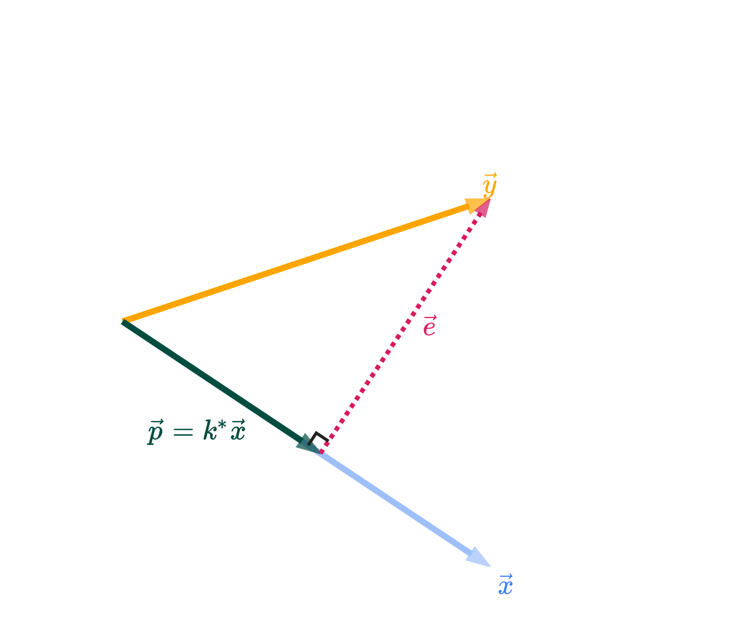
Among all vectors of the form kx, which one is closest to y?
We now know the answer is the vector p, where
p=(x⋅xy⋅x)x
p is called the orthogonal projection of y onto x.
Note that I’ve used y and x here rather than u and v, just to make the notation more consistent with the notation we’ll use as we move back into the world of machine learning.
In our original look at the approximation problem, we were approximating y using a scalar multiple of just a single vector, x. The set of all scalar multiples of x, denoted by span({x}), is a line in Rn.
Key idea: instead of projecting onto the subspace spanned by just a single vector, how might we project onto the subspace spanned by multiple vectors?
Equipped with our understanding of linear independence, spans, subspaces, and column spaces, we’re ready to tackle a more advanced version of the approximation problem.
All three statements at the bottom of the box above are asking the exact same question; I’ve presented all three forms so that you see more clearly how the ideas of spans, column spaces, and matrix-vector multiplication fit together. I will tend to refer to the latter two versions of the problem the most. In what follows, suppose X is an n×d matrix whose columns x(1), x(2), ..., x(d) are the building blocks we want to approximate y with.
First, let’s get the trivial case out of the way. Ify∈colsp(X), then the vector in colsp(X) that is closest to y is just y itself. If that’s the case, there exists some w such that y=Xw exactly. This w is unique only if X's columns are linearly independent; otherwise, there will be infinitely many good w’s.
But, that’s not the case I’m really interested in. I care more about when y is not in colsp(X). (Remember, this is the case we’re interested in when we’re doing linear regression: usually, it’s not possible to make our predictions 100% correct, and we’ll have to settle for some error.)
Then what?
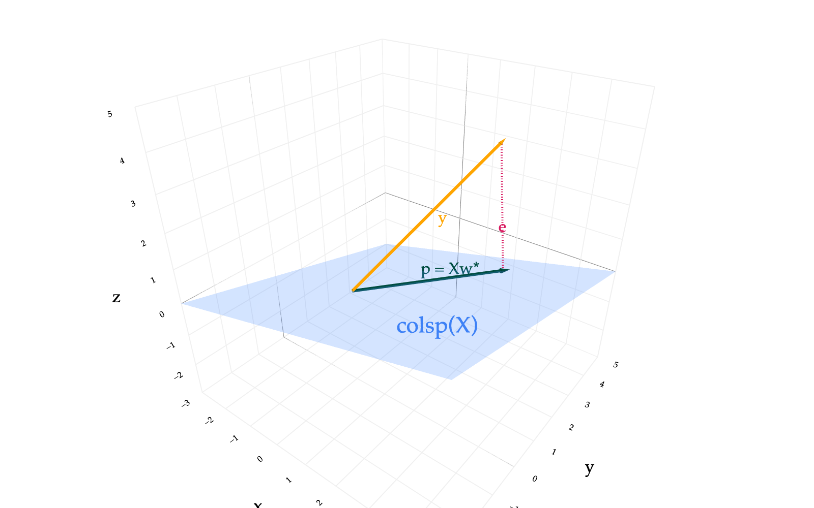
In general, colsp(X) is an r-dimensional subspace of Rn, where r=rank(X). In the diagram below, I’ve used a plane to represent colsp(X); just remember that X may have more than 3 rows or columns.
from utils import plot_vectors
import numpy as np
import plotly.graph_objects as go

y = np.array([1, 3, 2]) * 1.5
v1 = (1, 0, 0.25)
v2 = np.array([2, 2, 0]) * 0.5

def create_base_fig(show_spanners=True):
    # Define the vectors
    v3 = (-3.5 * v1[0] + 4 * v2[0], -3.5 * v1[1] + 4 * v2[1], -3.5 * v1[2] + 4 * v2[2])  # v3 is v1 + v2, which is on the plane spanned by v1 and v2

    # Plot the vectors using plot_vectors function
    vectors = [
        (tuple(y), "orange", "y"),
        (v1, "#3d81f6", "x⁽¹⁾"),
        (tuple(-v2), "#3d81f6", "x⁽²⁾"),
        (v3, "#3d81f6", "x⁽³⁾")
    ]

    if not show_spanners:
        vectors = [vectors[0]]

    fig = plot_vectors(vectors, show_axis_labels=True, vdeltaz=5, vdeltax=1)

    # Make the plane look more rectangular by using a smaller, symmetric range for s and t
    plane_extent = 20  # controls the "size" of the rectangle
    num_points = 3   # fewer points for a cleaner rectangle

    s_range = np.linspace(-plane_extent, plane_extent, num_points)
    t_range = np.linspace(-plane_extent, plane_extent, num_points)
    s_grid, t_grid = np.meshgrid(s_range, t_range)

    plane_x = s_grid * v1[0] + t_grid * v2[0]
    plane_y = s_grid * v1[1] + t_grid * v2[1]
    plane_z = s_grid * v1[2] + t_grid * v2[2]

    fig.add_trace(go.Surface(
        x=plane_x,
        y=plane_y,
        z=plane_z,
        opacity=0.8,
        colorscale=[[0, 'rgba(61,129,246,0.3)'], [1, 'rgba(61,129,246,0.3)']],
        showscale=False,
    ))

    # Annotate the plane with "colsp(X)"
    # Move the annotation "down" the plane by choosing negative s and t values
    label_s = 0.3
    label_t = 0.9
    label_x = label_s * v1[0] + label_t * v2[0]
    label_y_coord = label_s * v1[1] + label_t * v2[1] - 2
    label_z = label_s * v1[2] + label_t * v2[2]

    fig.add_trace(go.Scatter3d(
        x=[4],
        y=[-2],
        z=[2],  # small offset above the plane for visibility
        mode="text",
        text=[r"colsp(X)"],
        textposition="middle center",
        textfont=dict(size=22, color="#3d81f6"),
        showlegend=False
    ))

    # Set equal ranges for all axes to make grid boxes square
    axis_range = [-3, 5]  # Same range for all axes

    fig.update_layout(
        scene_camera=dict(
            eye=dict(x=1, y=-1.3, z=1)
        ),
        scene=dict(
            xaxis=dict(
                range=axis_range,
                dtick=1,
            ),
            yaxis=dict(
                range=axis_range,
                dtick=1,
            ),
            zaxis=dict(
                range=axis_range,
                dtick=1,
            ),
            aspectmode="cube",
            aspectratio=dict(x=1, y=1, z=1),  # Explicitly set 1:1:1 ratio
        ),
    )
    return fig

create_base_fig().show()
Loading...
Remember that colsp(X) is the set of linear combinations of X's columns, so it’s the set of all vectors that can be written as Xw, where w∈Rd.
Let’s consider two possible vectors of the form Xw, and look at their corresponding error vectors, e=y−Xw. I won’t draw the columns of X, since those would clutter up the picture.
def plot_vectors_with_errors(vectors_list, base_fig=None, notation="0"):
    """
    Takes a list of vectors and draws each one in #004d40 with a dotted error line in #d81a60.

    Parameters:
    -----------
    vectors_list : list of array-like
        List of vectors to plot. Each vector should be a 3D point/vector.
    base_fig : plotly.graph_objects.Figure, optional
        Base figure to build upon. If None, creates a new base figure using create_base_fig().

    Returns:
    --------
    fig : plotly.graph_objects.Figure
        The figure with vectors and error lines added.
    """
    fig = create_base_fig(show_spanners=False)

    # Get y vector from create_base_fig (defined the same way)
    y = np.array([1, 3, 2]) * 1.5

    for i, vec in enumerate(vectors_list):
        vec = np.array(vec)

        # Draw the vector in #004d40
        fig.add_trace(go.Scatter3d(
            x=[0, vec[0]],
            y=[0, vec[1]],
            z=[0, vec[2]],
            mode='lines',
            line=dict(color='#004d40', width=6),
            showlegend=False
        ))

        # Add arrowhead for the vector
        fig.add_trace(go.Cone(
            x=[vec[0]],
            y=[vec[1]],
            z=[vec[2]],
            u=[vec[0]],
            v=[vec[1]],
            w=[vec[2]],
            colorscale=[[0, '#004d40'], [1, '#004d40']],
            showscale=False,
            sizemode="absolute",
            sizeref=0.3,
            showlegend=False
        ))

        # Draw the error line (dotted) from vec to y in #d81a60
        fig.add_trace(go.Scatter3d(
            x=[vec[0], y[0]],
            y=[vec[1], y[1]],
            z=[vec[2], y[2]],
            mode='lines',
            line=dict(color='#d81a60', width=4, dash='dash'),
            showlegend=False
        ))

        # Annotate the vectors and error lines
        if i == 0:
            # Annotate the vector as Xw₀
            fig.add_trace(go.Scatter3d(
                x=[1], y=[3], z=[-0.5],
                mode='text',
                text=["p\u2080 = Xw\u2080"] if notation == "0" else ["p = Xw*"],  # \u2080 is Unicode subscript zero
                textposition="middle center",
                textfont=dict(color='#004d40', size=16),
                showlegend=False
            ))
            # Annotate the error as e₀
            mid_error = (vec + y) / 2
            fig.add_trace(go.Scatter3d(
                x=[mid_error[0]],
                y=[mid_error[1]],
                z=[mid_error[2]],
                mode='text',
                text=["e\u2080"] if notation == "0" else ["e"],
                textposition="bottom center",
                textfont=dict(color='#d81a60', size=16),
                showlegend=False
            ))
        else:
            # Annotate the vector as Xw'
            fig.add_trace(go.Scatter3d(
                x=[2], y=[-1], z=[1],
                mode='text',
                text=["p' = Xw'"],
                textposition="middle center",
                textfont=dict(color='#004d40', size=16),
                showlegend=False
            ))
            # Annotate the error as e'
            mid_error = (vec + y) / 2
            fig.add_trace(go.Scatter3d(
                x=[mid_error[0]],
                y=[mid_error[1]],
                z=[mid_error[2]],
                mode='text',
                text=["e'"],
                textposition="bottom center",
                textfont=dict(color='#d81a60', size=16),
                showlegend=False
            ))

    return fig

fig = create_base_fig()

# y = np.array([1, 3, 2]) * 1.5
# v1 = (1, 0, 0.25)
# v2 = np.array([2, 2, 0]) * 0.5

X = np.vstack([v1, v2]).T
w = np.linalg.inv(X.T @ X) @ X.T @ y
# w = [-1.333, 3.6667]
p = X @ w
other_p = X @ np.array([2, 1])

test_vectors = [p, other_p]

# Plot vectors with errors
fig = plot_vectors_with_errors(test_vectors, fig)
fig.show()
Loading...
Our problem boils down to finding the w that minimizes the norm of the error vector. Since it’s a bit easier to work with squared norms (remember that ∥x∥2=x⋅x), we’ll minimize the squared norm of the error vector instead; this is an equivalent problem, since the norm is non-negative to begin with.
which w minimizes this?∥e∥2=∥y−Xw∥2
Think of ∥y−Xw∥2 as a function of w only; X and y should be thought of as fixed. This is a least squares problem: we’re looking for the w that minimizes the sum of squared errors between y and Xw.
There are two ways we’ll minimize this function of w:
Using a geometric argument, as we did in the single vector case.
Using calculus. This is more involved than before, since the input variable is a vector, not a scalar, but it can be done, as we’ll see in Chapter 4.
Let’s focus on the geometric argument. What does our intuition tell us? Extending the single vector case, we expect the vector in colsp(X) that is closest to y to be the orthogonal projection of y onto colsp(X): that is, its error should be orthogonal to colsp(X).
We could see this intuitively in the visual above. wo was chosen to make eo orthogonal to colsp(X), meaning that eo is orthogonal to every vector in colsp(X). (The subscript “o” stands for “orthogonal”.) w′ was some other arbitrary vector, leading e′ to not be orthogonal to colsp(X). Clearly eo is shorter than e′.
To prove that the optimal choice of w comes from making the error vector orthogonal to colsp(X), you could use the same argument as in the single vector case: if you consider two vectors, wo with an orthogonal error vector eo, and w′ with an error vector e′ that is not orthogonal to colsp(X), then we can draw a right triangle with e′ as the hypotenuse and eo as one of the legs, making
∥e′∥2>∥eo∥2
This is such an important idea that I want to redraw the picture above with just the orthogonal projection. Note that I’ve replaced wo with w∗ to indicate that this is the optimal choice of w.
fig = create_base_fig()

# y = np.array([1, 3, 2]) * 1.5
# v1 = (1, 0, 0.25)
# v2 = np.array([2, 2, 0]) * 0.5

X = np.vstack([v1, v2]).T
w = np.linalg.inv(X.T @ X) @ X.T @ y
# w = [-1.333, 3.6667]
p = X @ w
test_vectors = [p]

# Plot vectors with errors and draw a right angle between p and e
fig = plot_vectors_with_errors(test_vectors, fig, notation='*')
fig.show(renderer='png', scale=2)
A Proof that the Orthogonal Error Vector is the Shortest
In office hours, a student asked for more justification that the shortest possible error vector is one that’s orthogonal to the column space of X, especially because it’s hard to visualize what orthogonality looks like in higher dimensions. Remember, all it means for two vectors to be orthogonal is that their dot product is 0.
Given that, let’s assume only that
wo is chosen so that eo=y−Xwo is orthogonal to colsp(X), and
w′ is any other choice of w, with a corresponding error vector e′=y−Xw′.
Just with these facts alone, we can show that eo is the shortest possible error vector. To do so, let’s start by considering the (squared) magnitude of e′:
∥e′∥2≥∥eo∥2=∥y−Xw′∥2=seems arbitrary, but it’s a legal operation that brings woback in∥y−Xw′+Xwo−Xwo∥2=∥‘‘a"y−Xwo+‘‘b"X(wo−w′)∥2=∥a+b∥2=∥a∥2+∥b∥2+2a⋅b∥y−Xwo∥2+∥X(wo−w′)∥2+2(y−Xwo)⋅X(wo−w′)=∥eo∥2+∥X(wo−w′)∥2+0, because eo is orthogonal to the columns of X2eo⋅X(wo−w′)=∥eo∥2+∥X(wo−w′)∥2
So, no matter what choice of w′ we make, the magnitude of e′ can’t be smaller than the magnitude of eo. This means that the error vector that is orthogonal to the column space of X is the shortest possible error vector.
This is really just the same proof as in Chapter 2.3, where we argued that eo, X(wo−w′), and e′ form a right triangle, where e′ is the hypotenuse.
We’ve come to the conclusion that in order to find the w that minimizes
∥e∥2=∥y−Xw∥2
we need to find the w that makes the error vector e=y−Xw orthogonal to colsp(X). colsp(X) is the set of all linear combinations of X's columns. So, if we can find an e that is orthogonal to every column of X, then it must be orthogonal to any of their linear combinations, too.
So, we’re looking for a e=y−Xw that satisfies
x(1)⋅(y−Xw)x(2)⋅(y−Xw)x(d)⋅(y−Xw)=0=0⋮=0
As you might have guessed, there’s an easier way to write these d equations simultaneously. Above, we’re taking the dot product of y−Xw with each of the columns of X. We’ve learned that Av contains the dot products of v with the rows of A. So how do we get the dot products of y−Xw with the columns of X? Transpose it!
So, if we want y−Xw to be orthogonal to each of the columns of X, then we need XT(y−Xw)=0 (note that this is the vector 0∈Rd, not the scalar 0.) Another way of saying this is that we need the error vector to be in the left null space of X, i.e. e∈null(XT).
XTeXT(y−Xw)XTy−XTXwXTXw=0=0=0=XTy
The final equation above is called the normal equation. “Normal” means “orthogonal”. Sometimes it’s called the normal equations to reference the fact that it’s a system of d equations and d unknowns, where the unknowns are components of w (w1,w2,…,wd.)
Note that XTXw=XTy looks a lot like Xw=y, with added factors of XT on the left. Remember that if y is in colsp(X), then Xw=y has a solution, but that’s usualy not the case, hence why we’re attempting to approximate y with a linear combination of X’s columns.
Is there a unique vector w that satisfies the normal equation? That depends on whether XTX is invertible. XTX is a d×d matrix with the same rank as the n×d matrix X, as we proved in Chapter 2.8.
rank(XTX)=rank(X)
So, XTX is invertible if and only if rank(X)=d, meaning all of X’s columns are linearly independent. In that case, the best choice of w is the unique vector
w∗=(XTX)−1XTy
w∗ has a star on it, denoting that it is the best choice of w. I don’t ask you to memorize much (you get to bring a notes sheet into your exams, after all), but this equation is perhaps the most important of the semester! It might even look familiar: back in the single vector case in Chapter 2.3, the optimal coefficient on x was x⋅xx⋅y=xTxxTy, which looks similar to the one above. The difference is that here, XTX is a matrix, not a scalar. (But, if X is just a matrix with a single column, then XTX is just the dot product of X with itself, which is a scalar, and the boxed formula above reduces to the formula from Chapter 2.3.)
What if XTXisn’t invertible? Then, there are infinitely many w∗'s that satisfy the normal equation,
XTXw=XTy
It’s not immediately obvious what it means for there to be infinitely many solutions to the normal equation; I’ve dedicated a whole subsection to it below to give this idea the consideration it deserves.
In the examples that follow, we’ll look at how to find all of the solutions to this equation when there are infinitely many.
First, let’s start with a straightforward example. Let
X=⎣⎡1210011−1⎦⎤,y=⎣⎡1045⎦⎤
The vector in colsp(X) that is closest to y is the vector Xw∗, where w∗ is the solution to the normal equations,
XTXw∗=XTy
The first step is to compute XTX, which is a 2×2 matrix of dot products of the columns of X.
XTX=[6333]
XTX is invertible, so we can solve for w∗ uniquely. Remember that in practice, we’d ask Python to solve np.linalg.solve(X.T @ X, X.T @ y), but here XTX is small enough that we can invert it by hand.
The magic is in the interpretation of the numbers in w∗, 2 and −38. These are the coefficients of the columns of X in the linear combination that is closest to y. Meaning,
Find the point on the plane 6x−3y+2z=0 that is closest to the point (1,1,1).
Solution
At first, this doesn’t seem like a projection problem, but it is. The plane
6x−3y+2z=0
is a 2-dimensional subspace of R3, meaning it can be described as the span of two non-collinear vectors. So, all we need to do is find some matrix X with those two vectors as columns, and then use the formula we derived above to project y=⎣⎡111⎦⎤ onto colsp(X). The fact that we said “point” instead of “vector” doesn’t change the problem: in settings like these, points and vectors are equivalent.
Two vectors that lie in the plane (but point in different directions) are ⎣⎡120⎦⎤ and ⎣⎡10−3⎦⎤. There’s nothing special about these two vectors, other than that they have relatively small integer components. Let’s use them as columns of X:
X=⎣⎡12010−3⎦⎤
Now, to formulate the normal equations, XTXw∗=XTy, we need to compute XTX and XTy.
XTX=[11200−3]⎣⎡12010−3⎦⎤=[51110]
XTy=[11200−3]⎣⎡111⎦⎤=[3−2]
So, the normal equations are
[51110]w∗[w0∗w1∗]=[3−2]
We could use w∗=(XTX)−1XTy, but often it’s easier to solve the system directly.
5w0∗+w1∗w0∗+10w1∗=3=−2
Solving this system gives us w0∗=4932 and w1∗=−4913. (Sorry, I know the numbers aren’t pretty in this example. But that’s what happens in the real world.)
Now that we’ve solved for w∗=[4932−4913], the projection of y onto colsp(X) – which is the point on the plane that’s closest to y – is
Find the orthogonal projection of y=⎣⎡132−1⎦⎤ onto colsp(X), where X=⎣⎡1210011−1⎦⎤.
Solution
First, notice that y is just the sum of the two columns of colsp(X). So intuitively, because y is already in the column space of X, the projection is just y itself.
The condition ZTeZ=[00] gives us some relationships involving e1,e2,e3,e4, but not enough to guarantee that the components sum to 0.
Key takeaway: Remember that XTeX=[00] implies that eX is orthogonal to any linear combination of the columns of X. So, if you can create a column of all 1’s using a linear combination of X’s columns, then the components of eX will sum to 0, no matter which vector y you choose to project onto colsp(X).
This is one of the most important consequences of orthogonal projections, especially as it relates to linear regression.
Usually, our data doesn’t come to us with orthogonal columns. But, using the Gram-Schmidt process introduced to you in Homework 7, you can convert a set of linearly independent vectors into an orthogonal set with the same span, allowing you to leverage that QTQ=I and simplify the projection process.
Key takeaway: Orthonormal vectors are very easy to work with!
In general, X is not a square matrix, so it can’t be invertible!
If X is square and invertible, then the steps above are valid. But, if X is a square and invertible n×n matrix, then colsp(X)=Rn, meaning that any y in Rn can be written as a linear combination of X’s columns, meaning that y is already in colsp(X), and there is no projection error (or need to do a projection in the first place).
In the case where X’s columns are linearly dependent, we can’t invert XTX to solve for w∗. This means that
XTXw=XTy
has infinitely many solutions. Let’s give more thought to what these solutions actually are.
First, note that all of these solutions for w∗correspond to the same projection,p=Xw∗. The “best approximation” of y in colsp(X) is always just one vector; if there are infinitely many w∗'s, that just means there are infinitely many ways of describing that one best approximation. This is because if vectors are linearly dependent, then their linear combinations aren’t unique, but if they are linearly independent, their linear combinations are unique.
Let me drive this point home further. Let’s suppose both w1 and w2 satisfy
XTXw=XTy
Then,
XTXw1−XTXw2=y−y=0
which means that
(XTX)(w1−w2)=0
i.e. the difference between the two vectors, w1−w2, is in nullsp(XTX). But, back in Chapter 2.8, we proved that XTX and X have the same null space, meaning any vector that gets sent to 0 by X also gets sent to 0 by XTX, and vice versa.
So,
X(w1−w2)=0
too, but that just means
Xw1=Xw2
meaning that even though w1 and w2 are different-looking coefficient vectors, they both still correspond to the same linear combination of X’s columns!
Let’s see how we can apply this to an example. Let X=⎣⎡363121010⎦⎤ and y=⎣⎡213⎦⎤. This is an example of a matrix with linearly dependent columns, so there’s no unique w∗ that satisfies the normal equations.
One way to find a possible vector w∗ is to solve the normal equations. XTX is not invertible, so we can’t solve for w∗ uniquely, but we can try and find a parameterized solution.
I’m going to take a different approach here: instead, let’s just toss out the linearly dependent columns of X and solve for w∗ using the remaining columns. Then, w∗ for the full X can use the same coefficients for the linearly independent columns, but 0s for the dependent ones. Removing the linearly dependent columns does not change colsp(X) (i.e. the set of all linear combinations of X’s columns), so the projection is the same.
The easy solution is to keep columns 2 and 3, since their numbers are smallest. So, for now, let’s say
X′=⎣⎡121010⎦⎤,y=⎣⎡213⎦⎤
Here, w′=(X′TX′)−1X′Ty=[5/2−4]. I won’t bore you with the calculations; you can verify them yourself.
Now, one possible w∗ for the full X is ⎣⎡05/2−4⎦⎤, which keeps the same coefficients on columns 2 and 3 as in w′, but 0 for the column we didn’t use.
As I mentioned above, if there are infinitely many solutions to the normal equation, then the difference between any two solutions is in nullsp(XTX), which is also nullsp(X). Put another way, if ws satisfies the normal equations, then so does ws+n for any n∈nullsp(XTX).
XTXwsXTX(ws+n)=XTy=XTXws+0, by definition of null spaceXTXn=XTy+0
So, once we have one w∗, to get the rest, just add any vector in nullsp(XTX) or nullsp(X) (since those are the same spaces).
What is nullsp(X)? It’s the set of vectors v such that Xv=0.
In our particular example,
X=⎣⎡363121010⎦⎤
we see that rank(X)=2, so nullsp(X) has a dimension of 3−2=1 (by the rank-nullity theorem), so it’s going to be the span of a single vector. All we need to do now is find one vector in nullsp(X), and we will know that the null space is the set of scalar multiples of that vector.
So, since nullsp(X)=nullsp(XTX)=span⎝⎛⎩⎨⎧⎣⎡1−30⎦⎤⎭⎬⎫⎠⎞, we know that the set of all possible w∗'s is
there are infinitely many solutions to the normal equations, but they’re all of this form⎣⎡05/2−4⎦⎤+t⎣⎡1−30⎦⎤,t∈R
This is not a subspace, since it doesn’t contain the zero vector.
There’s another way to arrive at this set of possible w∗'s: we can solve the normal equations directly. I wouldn’t recommend this second approach since it’s much longer, but I’ll add it here for completeness.
The first and second equations are just scalar multiples of each other, so we can disregard one of them, and solve for a form where we can use one unknown as a parameter for the other two. To illustrate, let’s pick w1∗=t.
18t+6w2∗+2w3∗6t+2w2∗+w3∗=7=1(2)(3)
(2)−3⋅(3) gives us w3∗=−4. Plugging this into both equations gives us
These are now both the same equation; the first one is just 3 times the second. So, we can solve for w2∗ in terms of t:
w2∗=25−6t
which gives us the complete solution
w∗=⎣⎡t25−6t−4⎦⎤,t∈R
This is the exact same line as using the null space approach! Plug in t=0 to get ⎣⎡05/2−4⎦⎤, for example. Again, this is not a subspace, since it doesn’t contain the zero vector.
So far, we’ve established that the vector in colsp(X) that is closest to y is the vector Xw∗, where w∗ is the solution to the normal equations,
XTXw∗=XTy
If XTX is invertible, then w∗ is the unique vector
w∗=(XTX)−1XTy
meaning that the vector in colsp(X) that is closest to y is
p=Xw∗=X(XTX)−1XTy
You’ll notice that the above expression also looks like a linear transformation applied to y, where y is being multiplied by the matrix
P=X(XTX)−1XT
The matrix P is called the projection matrix. In other classes, it is called the “hat matrix”, because they might use w^ instead of w∗ and y^ instead of p, and in that notation, y^=Py, so P puts a “hat” on y. (I don’t use hat notation in this class because drawing a hat on top of a vector is awkward. Doesn’t w^ look strange?)
So,
p=Xw∗=Py
shows us that there are two ways to interpret the act of projecting y onto colsp(X):
The resulting vector is some optimal linear combination of X's columns.
The resulting vector is the result of applying the linear transformation P to y.
Let’s work out an example. Suppose
X=⎣⎡30601540⎦⎤,y=⎣⎡123⎦⎤
X’s columns are linearly independent, so XTX is invertible, and
P=X(XTX)−1XT
is well-defined.
X = np.array([[3, 0],
              [0, 154],
              [6, 0]])

P = X @ np.linalg.inv(X.T @ X) @ X.T
P
P=⎣⎡0.200.40100.400.8⎦⎤ contains the information we need to project y onto colsp(X). Each row of P tells us the right mixture of y’s components we need to construct the projection.
Notice that P’s second row is [010]T. This came from the fact that X’s first column had a second component of 0 while its second column had a non-zero second component but zeros in the other two components, meaning that we can scale X’s second column to exactly match y’s second component. Change the 154 in X to any other non-zero value and P won’t change!
Additionally, if we consider some y that is already in colsp(X), then multiplying it by P doesn’t change it! For example, if we set y=⎣⎡31546⎦⎤ (the sum of X’s columns), then Py=y.
P @ np.array([3, 154, 6])
array([ 3., 154., 6.])
Let’s work through some examples that develop our intuition for P.
Suppose P=X(XTX)−1XT exists, meaning XTX is invertible. Is P invertible? If so, what is its inverse?
Solution
Before we do any calculations, intuitively the answer should be no. Once we’ve projected onto colsp(X), we’ve lost information, since we went from an arbitrary vector in Rn to a vector in a smaller subspace, so it shouldn’t be possible to reverse the projection. Put another way, two different vectors in Rn might have the same “shadow” onto colsp(X).
Even in the most recent example, P=⎣⎡0.200.40100.400.8⎦⎤ is not invertible, since column 3 is a multiple of column 1.
Let’s think about this a bit more from the perspective of ranks. It turns out that rank(P)=rank(X); I’ve provided a proof of this at the bottom of the solutions box, but you might want to attempt it on your own for practice.
Remember that X is an n×d matrix, meaning rank(X)≤min(n,d). X doesn’t need to have a rank of n for XTX to be invertible; it just needs to have a rank of d.
Since P is an n×n matrix, in general it won’t be the case that rank(P)=n. To illustrate, in the example above where P=⎣⎡0.200.40100.400.8⎦⎤, X was a 3×2 matrix with rank 2.
The only case in which rank(P)=n is when rank(X)=n, which also only happens when X is an n×n square matrix that is also invertible. In such a case, colsp(X)=Rn, and so we probably wouldn’t set out to project onto colsp(X) in the first place, since any vector in Rn is already a linear combination of X's columns.
Extra: Proof that rank(P)=rank(X)
We can show that this is the case by showing that P and X both have the same column spaces. This proof also helps explain why the normal equation, XTXw=XTy, always has at least one solution for w, even when XTX isn’t invertible.
Show colsp(P)⊆colsp(X), i.e. show that any vector in the column space of P is also in the column space of X.
If v∈colsp(P), then v can be written as a linear combination of P’s columns. Say v=Pu for some u∈Rn. Then,
v=Pu=Xsome vector((XTX)−1XTu)
Here, we see that if v=Pu, then v is also in X's column space. So,
v is a lin. comb. of P’s columns⟹v is a lin. comb. of X’s columns
Show colsp(X)⊆colsp(P), i.e. show that any vector in the column space of X is also in the column space of P.
This direction is a bit more involved. Let’s start by considering some vector v∈colsp(X), meaning
v=Xu
for some u∈Rd. What happens if we multiply both sides by P?
vPvPvPvPv=Xu=PXu=PX(XTX)−1XTXu=XI(XTX)−1XTXu=original definition of vXu=v
If v∈colsp(X), then v can be written as a linear combination of X's columns. Say v=Xw for some w∈Rd. Then,
v=Xw=Pw
So, if v=Xu, then v=Pv, meaning that v is also in P’s column space if it’s in X's column space. Intuitively, v=Pv means that if v is already in the span of X’s columns, then projecting it onto colsp(X) doesn’t change it.
Now that we’ve shown that colsp(P)⊆colsp(X) and colsp(X)⊆colsp(P), we can conclude that colsp(P)=colsp(X). If two sets are subsets of each other, then they must be equal.
No. Orthogonal matrices Q have the property that QTQ=QQT=I, meaning that
QT=Q−1
But, as we saw, P is not invertible in general, so it can’t satisfy this property. This tells us that Pdoes not perform a rotation; projections are not rotations. Rotations can be undone but projections can’t.
Yes. Symmetric matrices A have the property that AT=A. We can show that P satisfies this property; to do so, we’ll need to use the fact that (AB)T=BTAT.
PT=(X(XTX)−1XT)T=(XT)T((XTX)−1)TXT=X(XTX)−1XT=P
Going from the second to the third line, we used the fact that XTX is symmetric, and so is its inverse. Remember that XTX is a square matrix consisting of the dot products of the columns of X with themselves.
Intuitively, this means that P2y is the same as Py, meaning that once we’ve projected y onto colsp(X), projecting its projection p again onto colsp(X) gives us back the same p, since p is already in colsp(X).
Interpret PX as a matrix made up of Px(1), Px(2), ..., Px(d) as its columns. Px(i) is the projection of x(i) onto colsp(X), but since x(i) is already in colsp(X), projecting it again onto colsp(X) gives us back the same x(i). So, PX should just be X again.
Our goal is to find the linear combination of X’s columns that is closest to y.
This boils down to finding the vector w that minimizes ∥y−Xw∥2.
The vector w∗ that minimizes ∥y−Xw∥2 makes the resulting error vector, e=y−Xw∗, orthogonal to the columns of X.
The w∗ that makes the error vector orthogonal to the columns of X is the one that satisfies the normal equation,
XTXw∗=XTy
If XTX is invertible, which happens if and only if X’s columns are linearly independent, then w∗ is the unique vector
w∗=(XTX)−1XTy
otherwise, there are infinitely many solutions to the normal equation. All of these infinitely many solutions correspond to the same projection, p=Xw∗. If w′ is one solution (which can be found by removing the linearly dependent columns of X), then all other solutions are of the form w′+n, where n is any vector in nullsp(X)=nullsp(XTX).