2.4. Span and Linear Independence

$\color{#3d81f6}\vec v_1$ and $\color{#3d81f6}\vec v_2$ define a plane in $\mathbb{R}^3$. But not all pairs of vectors in $\mathbb{R}^3$ define a plane – for example, the vectors $\begin{bmatrix} 1 \\ 0 \\ 0 \end{bmatrix}$ and $\begin{bmatrix} 2 \\ 0 \\ 0 \end{bmatrix}$ define a line. How do we know if a set of vectors define a plane, line, or something else?

To motivate our discussion, let me recap “The Three Questions” involving linear combinations from Chapter 2.1.

So far, we’ve informally answered these questions in the context of various examples and problems. Here, I want to introduce a unifying framework for addressing these questions.

Above, I’ve used set builder notation to describe the span of a set of vectors. You’ll notice that I refer to $\vec v_1, \vec v_2, \ldots, \vec v_d$ as a set of vectors, but you’ll notice that I don’t always write them inside $\{ \text{set brackets} \}$; this is just to save space. But when referring to a span, I’ll always write the spanning set inside $\{ \text{set brackets} \}$.

Let’s look at several examples of spans, introducing important geometrical objects and ideas as we go. Chapter 2.5 will (eventually) cover how to describe lines, planes, and hyperplanes in $\mathbb{R}^n$, and is designed to complement this section.

Span of a Single Vector¶

Suppose we have just a single vector ${\color{#3d81f6}\vec v} \in \mathbb{R}^n$.

$\text{span}(\{{\color{#3d81f6}\vec v}\})$ is the set of all linear combinations of just $\color{#3d81f6}\vec v$. Since there is only vector in the spanning set, there aren’t any other vectors to add to $\color{#3d81f6}\vec v$, so the span is just the set of all scalar multiples of $\color{#3d81f6}\vec v$.

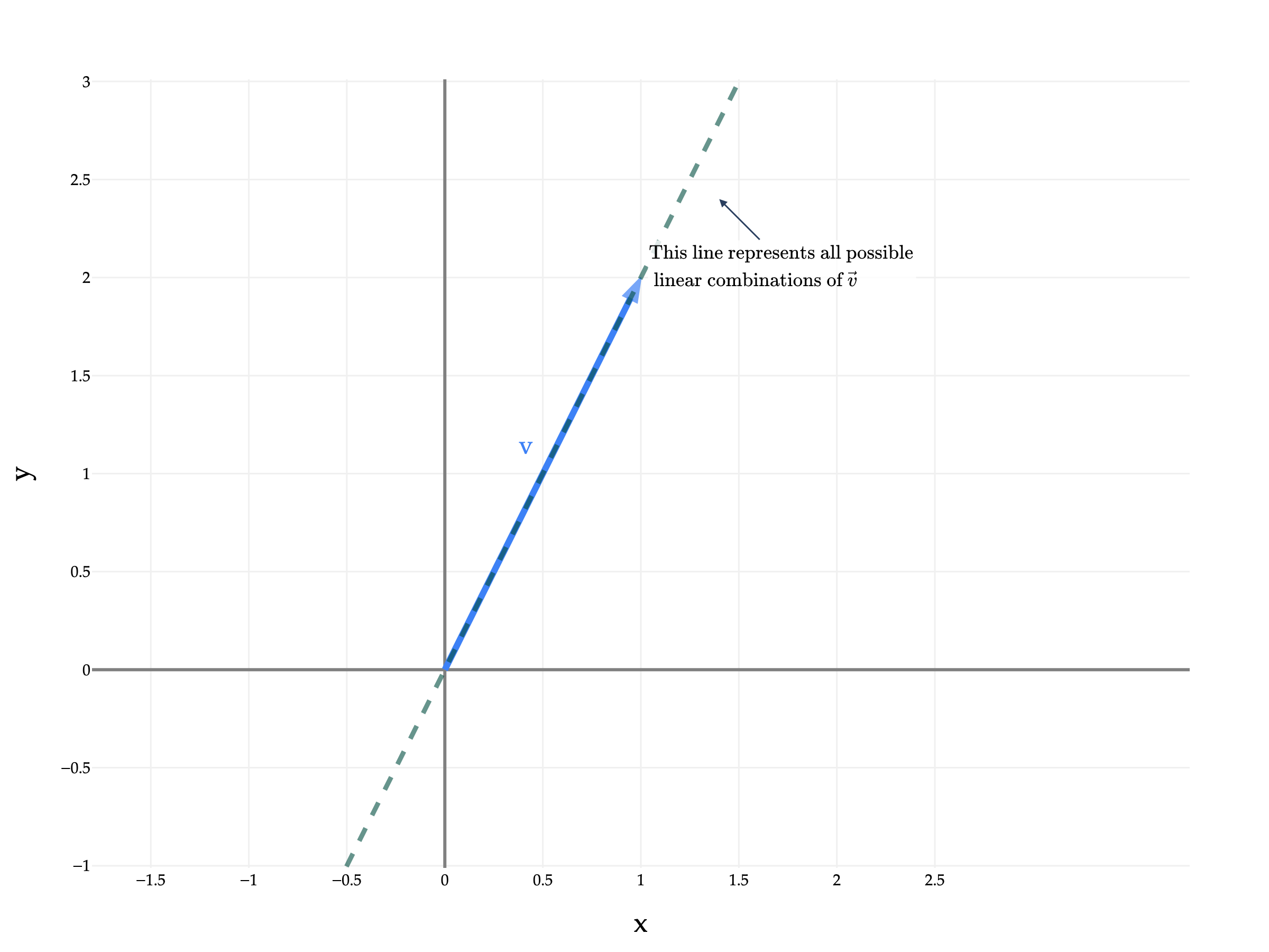
The span of a single vector is always a line that passes through the origin and the vector’s coordinates. Another way of saying this is that a single vector spans a line. In Chapter 2.3, we learned how to project one vector onto the span of another vector.

Example in $\mathbb{R}^2$¶

For example, if we consider $\color{#3d81f6}\vec v = \begin{bmatrix} 1 \\ 2 \end{bmatrix}$ in $\mathbb{R}^2$, the span is the line through the origin and $(1, 2)$, which you might also recognize as the line $y = 2x$.

There are infinitely many vectors in $\text{span}(\{{\color{#3d81f6} \begin{bmatrix} 1 \\ 2 \end{bmatrix}}\})$, including $\begin{bmatrix} 2 \\ 4 \end{bmatrix}$ and $\begin{bmatrix} -1 \\ -2 \end{bmatrix}$, and the line shown above contains all of them. Notationally, we could say

Example in $\mathbb{R}^3$¶

As another example, consider $\color{#3d81f6} \vec v = \begin{bmatrix} 2 \\ -1 \\ 3 \end{bmatrix}$ in $\mathbb{R}^3$. The span of $\color{#3d81f6} \vec v$ is the line through the origin and $(2, -1, 3)$.

The two marked points above are at the origin and $(2, -1, 3)$; I’ve marked them to emphasize that $\text{span}(\{{\color{#3d81f6} \begin{bmatrix} 2 \\ -1 \\ 3 \end{bmatrix}}\})$ is the unique line that passes through both $(2, -1, 3)$ and the origin. There are infinitely many lines that pass through $(2, -1, 3)$, but only one of those also passes through the origin.

Note that lines are 1-dimensional objects, regardless of the dimension of the space they live in. The line shown above is 1-dimensional in the sense that any point on the line can be described using a single variable. That variable is $a$ from the definition of the span:

Give me an $a$, and I’ll give you a point on the line.

Generalization to $\mathbb{R}^n$¶

The fact that a single vector spans a line is true, regardless of the dimension of the vectors themselves. The span of the vector $\begin{bmatrix} 1 \\ 2 \\ \vdots \\ 100 \end{bmatrix} \in \mathbb{R}^{100}$ is the line through the origin and $(1, 2, \ldots, 100)$ in $\mathbb{R}^{100}$. We can’t visualize what a line in 100-dimensional space looks like, but we know that it exists in this abstract sense.

Finally, I’ll say that in the edge case where $\color{#3d81f6}\vec v = \begin{bmatrix} 0 \\ 0 \\ \vdots \\ 0 \end{bmatrix} = \vec 0$, $\text{span}(\{{\color{#3d81f6} \vec 0}\}) = \left\{ {\color{#3d81f6} \vec 0} \right\}$ is just the single point corresponding to the origin, not a line.

To read more about how to describe lines in $\mathbb{R}^n$ – especially those that aren’t forced to pass through the origin, see Chapter 2.5.

Span of Two Vectors¶

Instead of considering just a single vector, let’s now consider the span of two vectors.

Examples in $\mathbb{R}^2$¶

Let’s start with a simple example: the span of two vectors in $\mathbb{R}^2$. Consider

$\text{span}(\{{\color{orange}\vec v_1}, {\color{#3d81f6}\vec v_2}\})$ is the set of all possible linear combinations of $\color{orange}\vec v_1$ and $\color{#3d81f6}\vec v_2$.

What is the set of all possible linear combinations of $\color{orange}\vec v_1$ and $\color{#3d81f6}\vec v_2$? Using $\color{orange}\vec v_1$ and $\color{#3d81f6}\vec v_2$ as building blocks, what are all possible vectors we can reach?

Since $\color{orange}\vec v_1$ and $\color{#3d81f6}\vec v_2$ point in different directions, we can reach any point in $\mathbb{R}^2$ by choosing appropriate values of $a_1$ and $a_2$.

So, if $\color{orange} \vec v_1 = \begin{bmatrix} 2 \\ 0 \end{bmatrix}$ and $\color{#3d81f6} \vec v_2 = \begin{bmatrix} 3 \\ 5 \end{bmatrix}$, $\text{span}(\{{\color{orange}\vec v_1}, {\color{#3d81f6}\vec v_2}\}) = \mathbb{R}^2$, meaning that $\color{orange} \vec v_1$ and $\color{#3d81f6} \vec v_2$ span the entire $xy$-plane.

Equivalently, for any vector $\vec b \in \mathbb{R}^2$, there exist $a_1$ and $a_2$ such that $a_1 {\color{orange}\vec v_1} + a_2 {\color{#3d81f6}\vec v_2} = \vec b$.

But, not every pair of vectors in $\mathbb{R}^2$ spans the entire plane. For example, consider the vectors

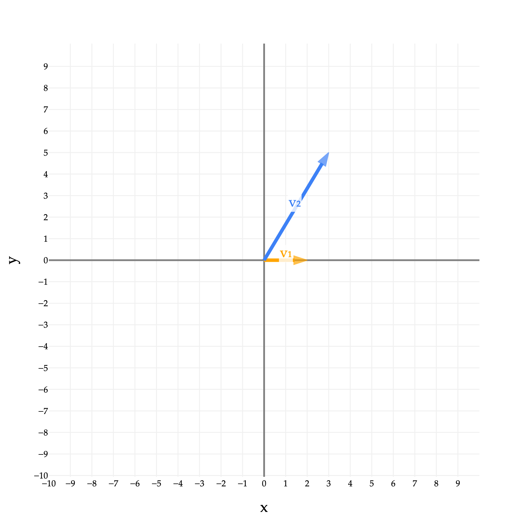
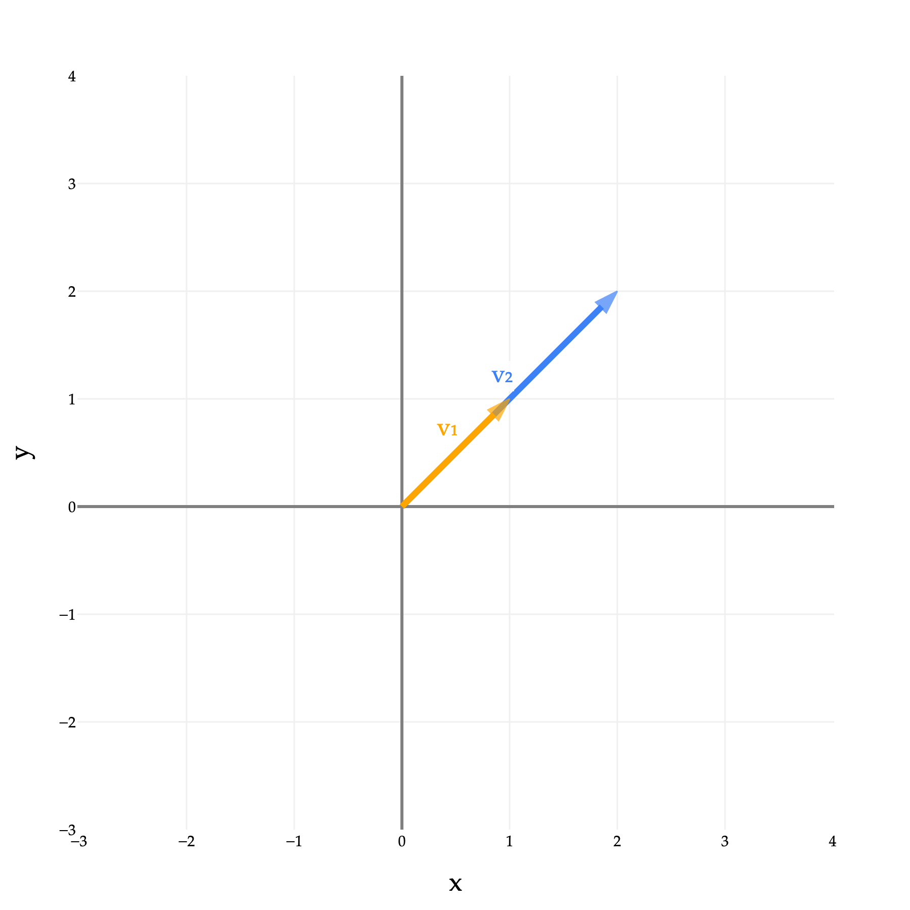
$\color{orange}\vec v_1$ and $\color{#3d81f6}\vec v_2$ are scalar multiples of each other – i.e. they are collinear – so they only span a line, despite there being two vectors. They span the same line that either one of them spans individually, which is the line through the origin, $(1, 1)$, and $(2, 2)$.

If we start with just $\color{orange}\vec v_1$, the vector $\color{#3d81f6}\vec v_2$ doesn’t “unlock” or “contribute” any new vectors to the span, since $\color{#3d81f6}\vec v_2$ is just a scalar multiple of $\color{orange}\vec v_1$. As we will soon see, this means that the vectors $\color{orange}\vec v_1$ and $\color{#3d81f6}\vec v_2$ are linearly dependent.

If we didn’t immediately recognize that $\color{#3d81f6}\vec v_2$ is just a scalar multiple of $\color{orange}\vec v_1$ and tried to write $\vec b = \begin{bmatrix} 8 \\ 11 \end{bmatrix}$ as a linear combination of $\color{orange}\vec v_1$ and $\color{#3d81f6}\vec v_2$, we might think it’s possible, since we’re working with a system of two equations and two unknowns.

But, when you go to solve, you’ll find

which is a contradiction, since $8 \neq 11$.

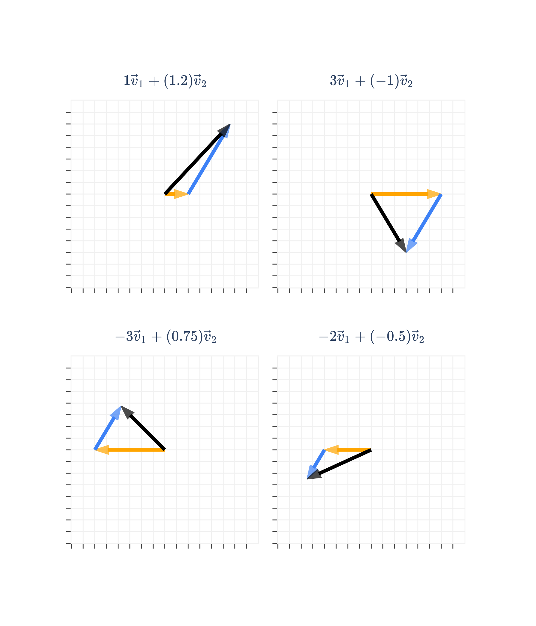
And, for the vectors $\vec b$ that are in $\text{span}(\{ {\color{orange}\vec v_1}, {\color{#3d81f6}\vec v_2} \})$, there are infinitely many ways to write them as linear combinations of $\color{orange}\vec v_1$ and $\color{#3d81f6}\vec v_2$. For example,

When solving for $a_1$ and $a_2$, I like to avoid situations where there are infinitely many solutions, since I’d like to make sure that if we all solve the same problem, we’ll all get the same answer. Remember that all of this connects back to linear regression and machine learning; the analog of $a_1$ and $a_2$ are the parameters of a linear model, and we’d like to have interpretable parameter values so that we can see how the inputs of a model relate to the outputs.

Back to the main idea. In $\mathbb{R}^2$, the span of two vectors is a line if the vectors are collinear, and the entire $xy$-plane otherwise.

Example in $\mathbb{R}^3$¶

Similar results hold for the span of two vectors in $\mathbb{R}^3$. Hopefully I’ve convinced you that

since $\begin{bmatrix} 10 \\ 4 \\ 2 \end{bmatrix}$ is just a scalar multiple of $\begin{bmatrix} 5 \\ 2 \\ 1 \end{bmatrix}$.

Let’s see a more interesting example. Consider the vectors

You’ll see them below, along with some of their linear combinations.

As was the case in $\mathbb{R}^2$, since $\color{orange} \vec v_1$ and $\color{#3d81f6} \vec v_2$ aren’t collinear, they span a plane. In $\mathbb{R}^2$, there was only one possible plane that two vectors could span, because all of $\mathbb{R}^2$ itself is a plane, but in $\mathbb{R}^3$ there are infinitely many planes.

A plane is a flat surface that extends infinitely in all directions, with the property that if you connect any two points on the plane, the line connecting them lies entirely on the plane.

So,

I hope to have convinced you earlier that lines are 1-dimensional objects, since you only need a single “variable” to describe any point on a given line.

Similarly, planes are 2-dimensional objects, since you need two “variables” to describe any point on a given plane. In the standard $xy$-plane, all you need to describe a point is an $x$ coordinate and a $y$ coordinate. Effectively, every vector in $\mathbb{R}^2$ can be written as a linear combination of the “default” (formally basis) vectors $\begin{bmatrix} 1 \\ 0 \end{bmatrix}$ and $\begin{bmatrix} 0 \\ 1 \end{bmatrix}$.

The plane shown above is also 2-dimensional, despite living in $\mathbb{R}^3$, since all I need are two variables to describe any point on it. The variables I need are $a_1$ and $a_2$, which are the multipliers on $\color{orange} \vec v_1$ and $\color{#3d81f6} \vec v_2$, respectively.

Think of $\color{orange} \vec v_1$ and $\color{#3d81f6} \vec v_2$ as defining a new coordinate system for the plane that they span, where the coordinates themselves are the scalars $a_1$ and $a_2$. $a_1$ and $a_2$ can be arbitrarily large or small, which is what allows the plane to extend infinitely.

The picture above makes clear that there are many vectors in $\text{span}(\{ {\color{orange} \vec v_1 }, {\color{#3d81f6} \vec v_2} \})$, but also many vectors in $\mathbb{R}^3$ that are not in the span. $a_1 {\color{orange} \vec v_1} + a_2 {\color{#3d81f6} \vec v_2} = \vec b$ has a solution for $a_1$ and $a_2$ if and only if $\vec b$ lies in the plane above.

In Chapter 2.5, I’ll say more about how to find the equation of a plane in the form $ax + by + cz + d = 0$, but that’s not particularly important to us right now.

Subspaces of $\mathbb{R}^n$¶

What if we’re dealing with two vectors in some arbitrary $\mathbb{R}^n$? Consider

These vectors live in $\mathbb{R}^5$, but what they span is a “plane” in $\mathbb{R}^5$. The more typical way of phrasing this is that these vectors span a 2-dimensional subspace of $\mathbb{R}^5$.

We will formally define vector spaces and subspaces in a later chapter, but for now, think of a subspace as a flat object that passes through the origin and contains all linear combinations of some set of vectors.

• A line through the origin is a 1-dimensional subspace.

• A plane through the origin is a 2-dimensional subspace.

• In higher dimensions, we’ll have 3-dimensional subspaces, 4-dimensional subspaces, and so on.

(A line that doesn’t pass through the origin is still a line, but isn’t a subspace, since subspaces must pass through the origin.)

The dimension of a subspace is the number of coordinates you need to describe any point in the subspace.

So although $\vec v_1 = \begin{bmatrix} 5 \\ 1 \\ 3 \\ 2 \\ -8 \end{bmatrix}$ and $\vec v_2 = \begin{bmatrix} 0 \\ 1 \\ 4 \\ 0 \\ 1 \end{bmatrix}$ sit inside $\mathbb{R}^5$, what they span is not all of $\mathbb{R}^5$, but rather a 2-dimensional “slice” of it, consisting of all linear combinations of $\vec v_1$ and $\vec v_2$. Any point in that subspace can be described using two coordinates, like $a_1$ and $a_2$ in

Span of Three Vectors¶

So far, as special cases, we’ve considered the span of one vector and the span of two vectors. The case of three vectors is the last special case I’ll cover, and then we’ll generalize to any number of vectors in any $\mathbb{R}^n$.

Examples in $\mathbb{R}^2$¶

Suppose we have three vectors in $\mathbb{R}^2$. What are their possible arrangements?

1. All three are the zero vector, $\vec 0$.

2. All three are collinear, meaning they lie on the same line.

3. Two are collinear, and the third points in a different direction.

4. All three point in different directions.

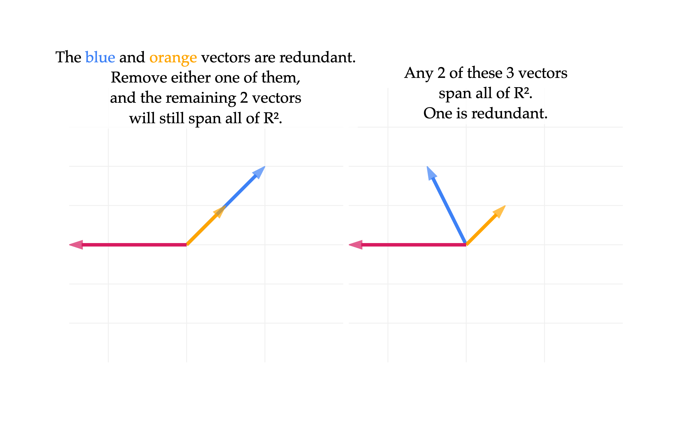
In all of these cases, the “largest” their span can be is all of $\mathbb{R}^2$. Case 3 and Case 4 are shown below, on the left and right, respectively.

In the left example, $\color{#d81b60} \vec v_3 = \begin{bmatrix} -3 \\ 0 \end{bmatrix}$ travels in a direction that $\color{orange} \vec v_1 = \begin{bmatrix} 1 \\ 1 \end{bmatrix}$ and $\color{#3d81f6} \vec v_2 = \begin{bmatrix} 2 \\ 2 \end{bmatrix}$ don’t, so removing $\color{#d81b60} \vec v_3$ would impact the span (it would drop from $\mathbb{R}^2$ to a line). But, we don’t need both $\color{orange} \vec v_1$ and $\color{#3d81f6} \vec v_2$ to span $\mathbb{R}^2$, since $\color{orange} \vec v_1$ already travels in the direction of $\color{#3d81f6} \vec v_2$.

In the right example, where

Any two of these vectors will span the entirety of $\mathbb{R}^2$, meaning that if you pick any two of them, you can recreate the third one. These three vectors are linearly dependent.

Examples in $\mathbb{R}^3$¶

Moving on up to $\mathbb{R}^3$, instead of considering all possible arrangements, let me enumerate their possible spans.

1. All three are the zero vector, $\vec 0$. (Annoying edge case, but I’m including it for completeness.)

2. All three are collinear, meaning they span a line.

3. All three are on the same plane, meaning they span that same plane.

4. None of the above, meaning they span all of $\mathbb{R}^3$.

As before, Case 1 and Case 2 are easy enough to reason about. First, let’s consider Case 3. Suppose

Notice that all three vectors lie on the same plane. But, as we saw earlier, you only need two vectors to span a plane. If you remove any one of the three vectors, the remaining two will still span the exact same plane.

This is a consequence of the fact that you can write ${\color{#d81b60}\vec v_3}$ as a linear combination of ${\color{orange}\vec v_1}$ and ${\color{#3d81f6}\vec v_2}$.

Starting from $\color{orange}\vec v_1$ and $\color{#3d81f6}\vec v_2$ alone, adding $\color{#d81b60}\vec v_3$ doesn’t unlock any new directions, since it’s already a linear combination of $\color{orange}\vec v_1$ and $\color{#3d81f6}\vec v_2$.

There is nothing “especially wrong” about $\color{#d81b60}\vec v_3$. We can rearrange the above to get ${\color{#3d81f6}\vec v_2} = -2{\color{orange}\vec v_1} - {\color{#d81b60}\vec v_3}$ and ${\color{orange}\vec v_1} = -\frac{1}{2}{\color{#3d81f6}\vec v_2} - \frac{1}{2}{\color{#d81b60}\vec v_3}$, too.

As we saw earlier in the case of two collinear vectors in $\mathbb{R}^2$, having a vector that can be written as a linear combination of the other vectors in the set means that when we go to write other vectors as linear combinations of the vectors in the set, if it’s possible, there are infinitely many solutions.

If we let $\vec b = \begin{bmatrix} b_1 \\ b_2 \\ b_3 \end{bmatrix}$ be any arbitrary vector in $\mathbb{R}^3$, then the system

either has no solutions, if $\vec b$ is not on the plane defined by $\text{span}(\{ {\color{orange}\vec v_1}, {\color{#3d81f6}\vec v_2}, {\color{#d81b60}\vec v_3} \})$, or it has infinitely many.

Let’s now consider Case 4, from the 4 cases above.

1. All three are the zero vector, $\vec 0$. (Annoying edge case, but I’m including it for completeness.)

2. All three are collinear, meaning they span a line.

3. All three are on the same plane, meaning they span that same plane.

4. None of the above, meaning they span all of $\mathbb{R}^3$.

Consider

Drag the plot around to see the space from different angles. If we look at any pair of these vectors, we see they span a plane. But, since neither is a linear combination of the other two, all three of them bring something new to the span; none are redundant.

So, the span of these three vectors is all of $\mathbb{R}^3$! You can think of these three vectors as defining a new coordinate system for $\mathbb{R}^3$.

The default coordinate system in $\mathbb{R}^3$ uses three numbers to describe any point in $\mathbb{R}^3$. Those three numbers are used to take a linear combination of the default basis vectors,

The coordinate system defined by $\color{orange}\vec v_1$, $\color{#3d81f6}\vec v_2$, and $\color{#d81b60}\vec v_3$ also uses three numbers to describe any point in $\mathbb{R}^3$, it’s just that the coordinates used multiply vectors other than the default ones.

So, any vector $\vec b \in \mathbb{R}^3$ can be written as a linear combination of $\color{orange}\vec v_1$, $\color{#3d81f6}\vec v_2$, and $\color{#d81b60}\vec v_3$.

Generalization to $\mathbb{R}^n$¶

Consider the following vectors in $\mathbb{R}^5$.

None of these vectors are a linear combination of the other two. So what do they span? A 3-dimensional subspace of $\mathbb{R}^5$.

That subspace is a 3-dimensional slice of the 5-dimensional space that is $\mathbb{R}^5$, and any vector in that subspace can be written using three coordinates.

If, say, $\vec v_3$ was a linear combination of $\vec v_1$ and $\vec v_2$, then the span would be a 2-dimensional subspace of $\mathbb{R}^5$.

Thinking in Higher Dimensions¶

Let’s generalize what we’ve discussed so far. What I’m about to say is abstract, but try and keep track of how it relates to the examples we’ve seen so far. If ever in doubt, plug in numbers for $d$ and $n$ to help make sense of it.

Remember that I’ve told you to think of a subspace as a flat object that passes through the origin and contains all linear combinations of some set of vectors. The dimension of a subspace is the number of coordinates you need to describe any point in the subspace; for instance, a line through the origin is a 1-dimensional subspace, and a plane through the origin is a 2-dimensional subspace.

Suppose we have $d$ vectors, all in $\mathbb{R}^n$, labeled $\color{#3d81f6}\vec v_1$, $\color{#3d81f6}\vec v_2$, ..., $\color{#3d81f6}\vec v_d$. Then,

• If we have fewer than $n$ vectors, i.e. $d < n$, then the vectors span a 1, or 2, or 3, ..., or $d$-dimensional subspace of $\mathbb{R}^n$.

• If we have at least $n$ vectors, i.e. $d \geq n$, then the vectors span a 1, or 2, or 3, ..., or $n$-dimensional subspace of $\mathbb{R}^n$. (An $n$-dimensional subspace of $\mathbb{R}^n$ is all of $\mathbb{R}^n$.)

Put this succinctly, the dimension of the subspace spanned by the vectors is between 1 and $\text{min}(d, n)$.

In general, given a set of $d$ vectors in $\mathbb{R}^n$, actually finding the dimension of the subspace they span involves solving a system of $n$ equations and $d$ unknowns. Later in this section, when we discuss how to find linear independent subsets, we’ll see how to do this by hand. But, know that numpy can help us.

For example, suppose we have $d = 5$ vectors in $\mathbb{R}^7$, given by

If we store all 5 vectors as arrays, and use the magical np.linalg.matrix_rank function, we get back the dimension of the subspace they span.

We’ll explore matrices soon. The rank of a matrix is the dimension of the subspace spanned by its columns.

Since np.linalg.matrix_rank returned 3, the vectors $\vec v_1, \vec v_2, \vec v_3, \vec v_4, \vec v_5$ span a 3-dimensional subspace of $\mathbb{R}^7$.

Linear Independence¶

There’s an idea we’ve implicitly been using for a while now but haven’t given a name to.

Definitions¶

Intuitively, if a set of vectors is linearly dependent, then one of the vectors is a linear combination of the others. Equivalently, if a set of vectors is linearly dependent, there’s a non-trivial linear combination of the vectors that equals the zero vector (by non-trivial, I mean that at least one of the coefficients is non-zero).

Why are these two conditions equivalent? Here’s one way to see it. Suppose $\vec v_1 = \alpha \vec v_2 + \beta \vec v_3$, meaning that $\vec v_1$ can be written as a linear combination of $\vec v_2$ and $\vec v_3$. Rearranging the equation above gives us

which shows us a non-trivial linear combination of $\vec v_1, \vec v_2, \vec v_3$ that gives $\vec 0$. The converse (reverse direction) is true too: if you start with a non-trivial linear combination of $\vec v_1, \vec v_2, \ldots, \vec v_d$ that gives $\vec 0$, then you can rearrange it to get $\vec v_1 = \text{some linear combination of } \vec v_2, \ldots, \vec v_d$.

Examples¶

Let’s look at several sets of vectors and comment on their linear independence (or lack thereof).

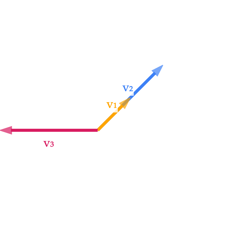
Note that if a set of vectors is linearly dependent, it doesn’t mean that every vector in the set can be written as a linear combination of the others. It just means that there’s at least one vector that can be written as a linear combination of the others. A good go-to example for this is the one below – $\color{orange} \vec v_1$ and $\color{#3d81f6} \vec v_2$ are scalar multiples of each other, making the entire set of three vectors linearly dependent, but but $\color{#d81b60} \vec v_3$ is not a linear combination of $\color{orange} \vec v_1$ and $\color{#3d81f6} \vec v_2$.

Unique Linear Combinations¶

Fact: If a set of vectors ${\color{#3d81f6}\vec v_1}, {\color{#3d81f6}\vec v_2}, \ldots, {\color{#3d81f6}\vec v_d}$ is linearly independent, then any vector $\vec b$ in the span of the vectors can be written as a unique linear combination of the vectors.

We’ve built intuition for this above, but let’s give a formal proof.

Let’s imagine an alternate universe where $\vec b \in \text{span}(\{{\color{#3d81f6}\vec v_1}, {\color{#3d81f6}\vec v_2}, \ldots, {\color{#3d81f6}\vec v_d}\})$ can be written as two different linear combinations of the vectors. (We’re doing a proof by contradiction, if you’re familiar with the idea.) In other words, suppose

and

and not all of the $a_i$ and $c_i$ are equal, meaning there’s at least one $i$ such that $a_i \neq c_i$.

What happens if we subtract the two equations?

Since ${\color{#3d81f6}\vec v_1}, {\color{#3d81f6}\vec v_2}, \ldots, {\color{#3d81f6}\vec v_d}$ are linearly independent, the only way this equation can hold is if all of the coefficients on the $\color{#3d81f6}\vec v_i$ are zero. In other words, we’d need

But if that’s the case, then $a_i = c_i$ for all $i$, which contradicts our assumption that not all of the $a_i$ and $c_i$ are equal.

So, this means that it can’t be the case that $\vec b$ can be written as two different linear combinations of the vectors. In other words, $\vec b$ can be written as a unique linear combination of the vectors, when the vectors ${\color{#3d81f6}\vec v_1}, {\color{#3d81f6}\vec v_2}, \ldots, {\color{#3d81f6}\vec v_d}$ are linearly independent.

Finding Linearly Independent Subsets with the Same Span¶

Given a set of vectors $\vec v_1, \vec v_2, \ldots, \vec v_d \in \mathbb{R}^n$, we’d like to find a subset of the vectors that is linearly independent and has the same span as the original set of vectors. In other words, we’d like to “drop” the vectors that are linearly dependent on the others. For example, if we have 3 vectors in $\mathbb{R}^3$ and they span a plane, we can drop one of them and still span the same plane (not just any plane).

In the example below, we can remove any one of the three vectors, and the span of the remaining two is still the same plane.

Dropping any “unnecessary” vectors will give us the desirable property that any vector in the span of the original set of vectors can be written as a unique linear combination of the vectors in the subset. (Remember that this has a connection to finding optimal model parameters in linear regression --- this is not just an arbitrary exercise in theory.)

One way to produce a linear independent subset is to execute the following algorithm:

given v_1, v_2, ..., v_d
initialize linearly independent set S = {v_1}
for i = 2 to d:
    if v_i is not a linear combination of S:
        add v_i to S

The vectors we’re left with form a basis for the span of the original set of vectors. The number of vectors we’re left with is the dimension of the span of the original set of vectors.

Let’s evaluate this algorithm on the following set of vectors:

First, we start with $\color{orange} S = \{\vec v_1\}$.

• Iteration 1 ($i = 2$): Is $\vec v_2$ a linear combination of the vectors in $S$?
  No, since $\vec v_2$ is not a multiple of $\vec v_1$. The first components (3 in $\vec v_1$, 0 in $\vec v_2$) imply that if $\vec v_2$ were a multiple of $\vec v_1$ it’d need to be $0 \vec v_1$, but the other components of $\vec v_2$ are non-zero.
  
  Outcome: Add $\vec v_2$ to $S$. Now, $\color{orange} S = \{\vec v_1, \vec v_2\}$.
  
  

• Iteration 2 ($i = 3$): Is $\vec v_3$ a linear combination of the vectors in $S$?
  To determine the answer, we need to try and find scalars $a_1$ and $a_2$ such that $a_1 \vec v_1 + a_2 \vec v_2 = \vec v_3$.

  $$a_1 \begin{bmatrix} 3 \\ 4 \\ 0 \end{bmatrix} + a_2 \begin{bmatrix} 0 \\ 1 \\ 1 \end{bmatrix} = \begin{bmatrix} -3 \\ -2 \\ 2 \end{bmatrix} \implies \begin{cases} 3a_1 + 0a_2 = -3 \\ 4a_1 + 1a_2 = -2 \\ 0a_1 + 1a_2 = 2 \end{cases}$$

  The first equation implies $a_1 = -1$ and the third equation implies $a_2 = 2$. Plugging both into the second equation gives $4(-1) + 1(2) = -2$, which is consistent. This means that $\vec v_3 = - \vec v_1 + 2 \vec v_2$, so $\vec v_3$ is a linear combination of $\vec v_1$ and $\vec v_2$, and we should not add it to $S$.
  
  Outcome: Leave $S$ unchanged. Now, $\color{orange} S = \{\vec v_1, \vec v_2\}$.
  
  

• Iteration 4 ($i = 4$): Is $\vec v_4$ a linear combination of the vectors in $S$?
  To determine the answer, we need to try and find scalars $a_1$ and $a_2$ such that $a_1 \vec v_1 + a_2 \vec v_2 = \vec v_4$.

  $$a_1 \begin{bmatrix} 3 \\ 4 \\ 0 \end{bmatrix} + a_2 \begin{bmatrix} 0 \\ 1 \\ 1 \end{bmatrix} = \begin{bmatrix} 6 \\ 5 \\ -3 \end{bmatrix} \implies \begin{cases} 3a_1 + 0a_2 = 6 \\ 4a_1 + 1a_2 = 5 \\ 0a_1 + 1a_2 = -3 \end{cases}$$

  Similarly, we see that $a_1 = 2$ (from the first equation) and $a_2 = -3$ (from the third equation) are consistent with the second equation. This means that $\vec v_4 = 2 \vec v_1 - 3 \vec v_2$, so $\vec v_4$ is a linear combination of $\vec v_1$ and $\vec v_2$, and we should not add it to $S$.
  
  Outcome: Leave $S$ unchanged. Now, $\color{orange} S = \{\vec v_1, \vec v_2\}$.
  
  

• Iteration 5 ($i = 5$): Is $\vec v_5$ a linear combination of the vectors in $S$?
  To determine the answer, we need to try and find scalars $a_1$ and $a_2$ such that $a_1 \vec v_1 + a_2 \vec v_2 = \vec v_5$.

  $$a_1 \begin{bmatrix} 3 \\ 4 \\ 0 \end{bmatrix} + a_2 \begin{bmatrix} 0 \\ 1 \\ 1 \end{bmatrix} = \begin{bmatrix} 2 \\ 5 \\ 1 \end{bmatrix} \implies \begin{cases} 3a_1 + 0a_2 = 2 \\ 4a_1 + 1a_2 = 5 \\ 0a_1 + 1a_2 = 1 \end{cases}$$

  The first equation implies $a_1 = \frac{2}{3}$ and the third equation implies $a_2 = 1$. Plugging both into the second equation gives $4(\frac{2}{3}) + 1(1) = \frac{11}{3} \neq 5$, which means the system is inconsistent. So, $\vec v_5$ is not a linear combination of $\vec v_1$ and $\vec v_2$, and we should add it to $S$.
  
  Outcome: Add $\vec v_5$ to $S$. Now, $\color{orange} S = \{\vec v_1, \vec v_2, \vec v_5\}$.